This page was generated from examples/ConsWealthUtilityModel/WealthUtilityConsumerType.ipynb.
Interactive online version: . Download notebook.

Wealth-in-Utility Multiplicatively with Consumption

The typical consumption-saving model assumes that agents derive a flow of utility from consumption each period, with additively separable utility across time. In HARK.ConsumptionSaving.ConsWealthUtility module, we change this assumption to allow wealth (end-of-period assets) to enter the agent’s utility function directly.

This notebook concerns agents whose direct preferences for wealth are represented multiplicatively with consumption under a Cobb-Douglas aggregator. For additive direct preferences for wealth, see the notebook for ``CapitalistSpiritConsumerType` <./CapitalistSpiritConsumerType.ipynb>`__ in the same module.

# Import basic packages and the AgentType subclass of interest
import matplotlib.pyplot as plt
from HARK.utilities import plot_funcs
from time import time

from HARK.ConsumptionSaving.ConsWealthUtilityModel import (
    WealthUtilityConsumerType,
    init_wealth_utility,
)
from HARK.ConsumptionSaving.ConsIndShockModel import IndShockConsumerType  # comparitor


def mystr(x):
    return "{:.4f}".format(x)

\[\newcommand{\R}{\mathbb{R}} \newcommand{\CRRA}{\rho} \newcommand{\LivPrb}{\mathsf{S}} \newcommand{\PermGroFac}{\Gamma} \newcommand{\Rfree}{\mathsf{R}} \newcommand{\DiscFac}{\beta} \newcommand{\WealthShare}{\alpha} \newcommand{\WealthShift}{\xi} \newcommand{\cNrm}{c} \newcommand{\mNrm}{m} \newcommand{\aNrm}{a}\]

Multiplicative Wealth-in-Utility Consumption-Saving Model Statement

A WealthUtilityConsumerType’s problem can be expressed as:

\[\begin{equation*} v_t(m_t) = \max_{c_t}u(x_t) + \DiscFac \LivPrb_{t} \mathbb{E}_{t} \left[ (\PermGroFac_{t+1} \psi_{t+1})^{1-\CRRA} v_{t+1}(m_{t+1}) \right] ~~\text{s.t.} \end{equation*}\]

\[\begin{split}\begin{eqnarray*} u(x) &=& \frac{x^{1-\CRRA}}{1-\CRRA}, \\ x_t &=& (a_t + \WealthShift)^\WealthShare c_t^{1-\WealthShare}, \\ a_t &=& m_t - c_t, \\ a_t &\geq& \underline{a}, \\ m_{t+1} &=& a_t \Rfree_{t+1}/(\PermGroFac_{t+1} \psi_{t+1}) + \theta_{t+1}, \\ (\psi_{t+1},\theta_{t+1}) &\sim& F_{t+1}, \\ \mathbb{E}[\psi] &=& 1. \\ \end{eqnarray*}\end{split}\]

This model is identical to that of an IndShockConsumerType but for the presence of the Cobb-Douglas combination of assets and consumption to yield “effective consumption” \(x_t\). As such, this model degenerates to IndShockConsumerType as \(\WealthShare \rightarrow 0\).

Note that the shifter term \(\WealthShift\) (denoted WealthShift in the model code) does not have a consistent interpretation in this normalized framework. That is, if \(\WealthShift > 0\), then the model above cannot be “de-normalized” to express preferences strictly in terms of levels of consumption and wealth. The model can still be solved when WealthShift is not zero, but the parameter will not control the extent to which wealth accumulation is a luxury good in levels.

NB: The HARK team will soon add a non-normalized version of this model to allow \(\WealthShift > 0\) to be interpreted consistently in levels.

Solving the Multiplicative Wealth-in-Utility Model

(This section is adapted from Appendix A.3 of “Life-Cycle Modeling is Ready for Prime Time”, which Matt White wrote.)

In the standard consumption-saving model with CRRA utility over consumption only, the first order condition w.r.t consumption is trivial to invert; this is not the case when consumption and wealth are multiplicatively combined into a single term in the CRRA function. To start, we substitute the Cobb-Douglas aggregator into the CRRA utility function:

\[\begin{split}\begin{eqnarray*} u(\cNrm, \aNrm) &=& \frac{\left(\cNrm^{1-\WealthShare}(\aNrm+\WealthShift)^{\WealthShare}\right)^{1-\CRRA}}{1-\CRRA} \\ &=& \frac{\left(\cNrm^{1-\WealthShare}(\mNrm - \cNrm + \WealthShift)^{\WealthShare}\right)^{1-\CRRA}}{1-\CRRA}. \end{eqnarray*}\end{split}\]

Fixing market resources \(\mNrm\) at some value of interest, the marginal return to utility from consumption is:

\[\begin{split}\begin{align*} \frac{\text{d}}{\text{d} \cNrm} u(\cNrm, \mNrm-\cNrm) &= \left[ (1-\WealthShare) \cNrm^{-\WealthShare} (\mNrm - \cNrm + \WealthShift)^\WealthShare - \WealthShare \cNrm^{1-\WealthShare}(\mNrm - \cNrm + \WealthShift)^{\WealthShare-1} \right] \cdot \left( (\mNrm - \cNrm + \WealthShift)^\WealthShare \cNrm^{1-\WealthShare} \right)^{-\CRRA} \\ &= \left[ (1-\WealthShare) \left(\frac{\cNrm}{\mNrm-\cNrm + \WealthShift}\right)^{-\WealthShare} - \WealthShare \left(\frac{\cNrm}{\mNrm - \cNrm + \WealthShift} \right)^{1-\WealthShare} \right] \cdot \left( (\mNrm - \cNrm + \WealthShift)^\WealthShare \cNrm^{1-\WealthShare} \right)^{-\CRRA} \\ &= \left[ (1-\WealthShare) \left(\frac{\cNrm}{\aNrm + \WealthShift}\right)^{-\WealthShare} - \WealthShare \left(\frac{\cNrm}{\aNrm + \WealthShift} \right)^{1-\WealthShare} \right] \cdot \left( (\aNrm + \WealthShift) (\aNrm + \WealthShift)^{\WealthShare-1} \cNrm^{1-\WealthShare} \right)^{-\CRRA} \\ &= \left[ (1-\WealthShare) \chi^{-\WealthShare} - \WealthShare \chi^{1-\WealthShare} \right] \cdot \left( (\aNrm + \WealthShift) \chi^{1-\WealthShare} \right)^{-\CRRA}, ~~~~ \chi \equiv \frac{\cNrm}{\aNrm + \WealthShift}. \end{align*}\end{split}\]

These algebraic manipulations will prove useful when we solve the first order condition momentarily. With wealth-in-utility preferences, the agent’s optimal consumption problem is:

\[\begin{align*} v_t(\mNrm_t) &= \max_\cNrm \left[ u(\cNrm, \mNrm_t-\cNrm) + \mathfrak{v}_t(\mNrm_t - \cNrm) \right]. \end{align*}\]

In this equation, we have already expressed the continuation or end-of-period value function over assets \(a_t\) in EGM form (see here), denoted as \(\mathfrak{v}_t(a_t)\).

Consider the first order condition for optimality by taking the derivative of the maximand with respect to \(\cNrm\) and equating it to zero:

\[\begin{equation} \frac{\text{d}}{\text{d} \cNrm} u(\cNrm_t, \mNrm_t-\cNrm_t) - \mathfrak{v}'_t(\mNrm_t - \cNrm_t) = 0. \end{equation}\]

We can substitute the final form of the marginal return to consumption, move the second term to the right-hand side, and then rearrange slightly to get:

\[\begin{equation*} \left[ (1-\WealthShare) \chi_t^{-\WealthShare} - \WealthShare \chi_t^{1-\WealthShare} \right] \cdot \left( (\aNrm_t + \WealthShift) \chi_t^{1-\WealthShare} \right)^{-\CRRA} = \mathfrak{v}'_t(\aNrm_t) \Longrightarrow \end{equation*}\]

\[\begin{equation*} \left[ (1-\WealthShare) \chi_t^{-\WealthShare} - \WealthShare \chi_t^{1-\WealthShare} \right]^{-1/\CRRA} \cdot \chi_t^{1-\WealthShare} = \underbrace{\mathfrak{v}'_t(\aNrm_t)^{-1/\CRRA} / (\aNrm_t + \WealthShift)}_{\equiv ~ \omega_t}. \end{equation*}\]

The left-hand side of the rearranged FOC is monotonically increasing with respect to \(\chi = \cNrm/(\aNrm+\WealthShift) > 0\), starting from zero and growing without bound. Moreover, the RHS (which uses only information about the continuation value through \(\aNrm_t\)) must be strictly positive, as both marginal value and end-of-period assets are strictly positive (the consumer will never choose \(\aNrm \leq -\WealthShift\) with these preferences because it would yield infinitely negative utility). Hence the first order condition has a unique solution in \(\chi_t\) for each \(\aNrm_t\).

Unfortunately, there is no closed form solution for the rearranged FOC to recover \(\chi_t\) from \(\omega_t\). While it would be possible to use a rootfinder to solve it for each value of \(\omega_t\) as it comes up during the solution process, it is more efficient to pre-compute a function that accurately maps from \(\omega\) to \(\chi\). We now describe a method for constructing such a function by working with the inverse relationship.

First, note that the expression in square brackets is not positive for all values of \(\chi > 0\), with the bounding condition defined by:

\[\begin{equation*} (1-\WealthShare) \chi^{-\WealthShare} - \WealthShare \chi^{1-\WealthShare} > 0 \Longrightarrow (1-\WealthShare) \chi^{-\WealthShare} > \WealthShare \chi^{1-\WealthShare} \Longrightarrow \frac{1-\WealthShare}{\WealthShare} >\chi. \end{equation*}\]

The expression in square brackets is raised to a negative power, hence we need only to consider values of \(\chi \in (0, (1 -\WealthShare)/\WealthShare)\). These \(\chi\) values represent the range of the function that maps from \(\omega\) to \(\chi\), and we want our constructed approximation to cover as much of that range as possible. To do so, we will use the logit transformation to map from an auxiliary variable \(z \in \R\) to \(\chi \in (0, (1 -\WealthShare)/\WealthShare)\):

\[\begin{equation*} \chi = \frac{\exp(z)}{1 + \exp(z)} \cdot \frac{1-\WealthShare}{\WealthShare}. \end{equation*}\]

The domain of the function we want to approximate is \(\omega > 0\) or \(\omega \in \R_{++}\), so we can work with \(\log(\omega)\) to ensure that we are working with strictly positive numbers. To approximate the mapping from \(\omega\) to \(\chi\):

1. Fix a grid of \(z\) values centered around zero; we use a uniformly spaced grid with 301 gridpoints between \(\pm 15\).

2. For each \(z\) in the grid, calculate the corresponding \(\chi\) using the logit transform. With our \(z\) grid, this spans the inner 99.99994% of the feasible range of \(\chi\).

3. For each \(\chi\) in that grid, calculate \(\omega\) using the rearranged FOC, then compute \(\log(\omega)\).

4. Construct a linear spline interpolant that maps from the vector of \(\log(\omega)\) values to the grid of \(z\), with linear extrapolation above and below; call this function \(g(\cdot)\).

5. Define function \(f(\cdot)\) as the composition of the logit transform, \(g\), and \(\log\).

By construction, \(f\) is an approximation of the mapping from \(\omega\) to \(\chi\) implicitly defined by the FOC, by successively applying the logarithm to \(\omega\), the interpolant from \(\log(\omega)\) to \(z\), and the logit transformation to recover \(\chi\). The approximation is extremely accurate, even on the extrapolated region on \(\omega\), because the underlying mapping from \(\log(\omega)\) to \(z\) approaches linearity on both ends. Conveniently, the \(f\) function depends on only \(\CRRA\) and \(\WealthShare\) and can be constructed once for all periods of the life-cycle.

In the HARK code, the \(f\) function is represented by an instance of the class ChiFromOmegaFunction, which is built by the constructor function make_ChiFromOmega_function.

With the mapping \(f : \omega \rightarrow \chi\) in hand, we can now describe our algorithm for solving for optimal consumption under wealth-in-utility preferences:

1. Fix an exogenous grid of \(\aNrm_t\) values from the natural borrowing constraint to a large value (say, a wealth-to-income ratio of 100).

2. For each \(\aNrm\) in the grid, evaluate \(\mathfrak{v}'_t(\aNrm_t)\), then raise it to the \(-1/\CRRA\) power and divide by \((\aNrm + \WealthShift)\), yielding a vector of \(\omega\) values.

3. For each \(\omega\) in that vector, compute \(\chi = f(\omega)\), then multiply by \((\aNrm + \WealthShift)\) to recover the optimal \(\cNrm\).

4. Find the associated decision-time state by inverting the intraperiod budget: \(\mNrm_t = \aNrm_t + \cNrm_t\).

5. Construct the consumption function as a linear interpolant over those \((\mNrm_t, \cNrm_t)\) pairs, adding a point at \(c_t=0\) corresponding to the natural borrowing constraint.

6. Construct the marginal value function \(v'_t(\mNrm_t)\) as the composition of the marginal utility function and the consumption function.

As a final note, the natural borrowing constraint in the wealth-in-utility is the more restrictive of the usual natural borrowing constraint (the lowest value of \(\aNrm_t\) such that a valid \(\mNrm_{t+1}\) value is reached no matter which income shocks realize) and \(-\WealthShift\). As mentioned above, utility flow goes to negative infinity (or at least marginal utility goes to positive infinity) as \(\aNrm_t \rightarrow -\WealthShift\) because of the Cobb-Douglas aggregator. Thus the agent will never choose to end the period with \(\aNrm_t \leq -\WealthShift\), so the natural borrowing constraint can be no lower than this level.

In the typical case with \(\WealthShift = 0\) in the permanent-income-normalized model, the agents will never borrow at all, even without an artificial liquidity constraint.

Example parameter values to construct a WealthUtilityConsumerType

The WealthUtilityConsumerType builds off of IndShockConsumerType, so the set of parameters that specify an instance (with default constructors) is very similar to the base class. The table below presents the complete list of parameters for WealthUtilityConsumerType, along with example values.

Parameter	Description	Code	Example value	Time-varying?
\(\DiscFac\)	Intertemporal discount factor	DiscFac	\(0.96\)
\(\CRRA\)	Coefficient of relative risk aversion	CRRA	\(2.0\)
\(\WealthShare\)	Share of wealth in Cobb-Douglas combination	WealthShare	\(0.2\)
\(\WealthShift\)	Additive shifter for wealth in Cobb-Douglas combination	WealthShift	\(0.0\)
\(\Rfree_t\)	Risk free interest factor	Rfree	\([1.03]\)	\(\surd\)
\(\LivPrb_t\)	Survival probability	LivPrb	\([0.98]\)	\(\surd\)
\(\PermGroFac_{t+1}\)	Permanent income growth factor	PermGroFac	\([1.01]\)	\(\surd\)
\(\sigma_\psi\)	Standard deviation of log permanent income shocks	PermShkStd	\([0.1]\)	\(\surd\)
\(N_\psi\)	Number of discrete permanent income shocks	PermShkCount	\(7\)
\(\sigma_\theta\)	Standard deviation of log transitory income shocks	TranShkStd	\([0.2]\)	\(\surd\)
\(N_\theta\)	Number of discrete transitory income shocks	TranShkCount	\(7\)
\(\mho\)	Probability of being unemployed and getting \(\theta=\underline{\theta}\)	UnempPrb	\(0.05\)
\(\underline{\theta}\)	Transitory shock when unemployed	IncUnemp	\(0.3\)
\(\mho^{Ret}\)	Probability of being “unemployed” when retired	UnempPrbRet	\(0.0005\)
\(\underline{\theta}^{Ret}\)	Transitory shock when “unemployed” and retired	IncUnempRet	\(0.0\)
\((none)\)	Period of the lifecycle model when retirement begins	T_retire	\(0\)
\((none)\)	Minimum value in assets-above-minimum grid	aXtraMin	\(0.001\)
\((none)\)	Maximum value in assets-above-minimum grid	aXtraMax	\(20.0\)
\((none)\)	Number of points in base assets-above-minimum grid	aXtraCount	\(48\)
\((none)\)	Exponential nesting factor for base assets-above-minimum grid	aXtraNestFac	\(3\)
\((none)\)	Additional values to add to assets-above-minimum grid	aXtraExtra	\(None\)
\(\underline{a}\)	Artificial borrowing constraint (normalized)	BoroCnstArt	\(0.0\)
\((none)\)	Indicator for whether vFunc should be computed	vFuncBool	\(True\)
\((none)\)	Indicator for whether cFunc should use cubic splines	CubicBool	\(False\)
\(T\)	Number of periods in this type’s “cycle”	T_cycle	\(1\)
(none)	Number of times the “cycle” occurs	cycles	\(0\)

Example Implementations of WealthUtilityConsumerType

The WealthUtilityConsumerType has workable defaults, so let’s begin with those, solving an infinite horizon problem right off the shelf. At the default parameters, WealthShare is \(0.2\) and WealthShift is \(0.0\).

# Make an infinite horizon wealth-in-utility consumer type with default parameters
WIUtype = WealthUtilityConsumerType(cycles=0)

# Solve the wealth-in-utility model
t0 = time()
WIUtype.solve()
t1 = time()
print(
    "Solving a wealth-in-utility consumption-saving problem took "
    + mystr(t1 - t0)
    + " seconds."
)

Solving a wealth-in-utility consumption-saving problem took 0.1080 seconds.

# Plot the consumption function
WIUtype.unpack("cFunc")
plt.ylim(0.0, 1.75)
plt.xlabel(r"Normalized market resources $m_t$")
plt.ylabel(r"Normalized consumption $c_t$")
plot_funcs(WIUtype.cFunc, 0.0, 10.0)

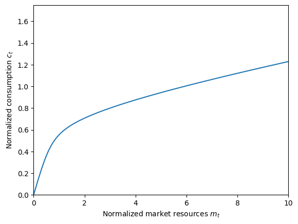
The consumption function for a WealthUtilityConsumerType will always be strictly less than the corresponding IndShockConsumerType, as long as WealthShare is positive. To see an example of this, let’s make an IndShockConsumerType with the same parameters as a default WealthUtilityConsumerType and compare their solutions.

# Make a basic consumer representation using the default parameters for the wealth-in-utility model
BaseType = IndShockConsumerType(**init_wealth_utility)
BaseType.assign_parameters(cycles=0)

# Solve the infinite horizon consumption-saving model for the standard model
t0 = time()
BaseType.solve()
t1 = time()
print(
    "Solving a standard consumption-saving problem took " + mystr(t1 - t0) + " seconds."
)

Solving a standard consumption-saving problem took 0.1040 seconds.

# Plot the consumption function for both types on the same figure
BaseType.unpack("cFunc")
plt.ylim(0.0, 1.75)
plt.xlabel(r"Normalized market resources $m_t$")
plt.ylabel(r"Normalized consumption $c_t$")
plot_funcs([WIUtype.cFunc[0], BaseType.cFunc[0]], 0.0, 10.0)

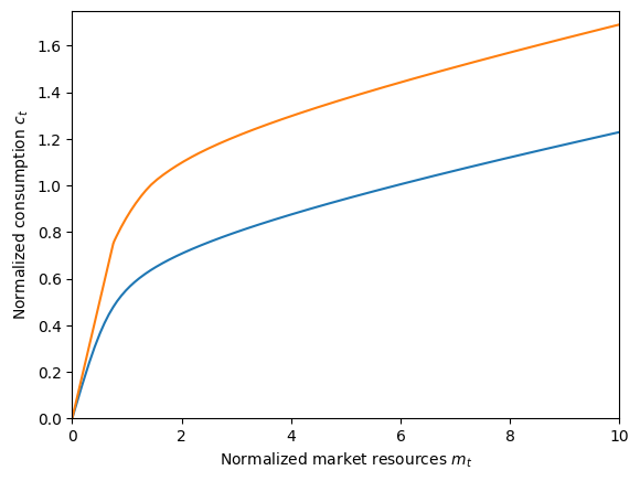
This graph illuminates one of the key features of the wealth-in-utility model: even though the agent is guaranteed to have strictly positive income in \(t+1\), they never want to end the period with \(a_t=0\), because this would yield infinitely negative utility. That is, the artificial borrowing constraint \(a_t \geq 0\) doesn’t bind.

To have the artificial borrowing constraint bind at low levels of \(m_t\), we can set \(\WealthShift > 0\) so that the agent is willing to go as low as \(a_t = -\WealthShift\) (but they’ll be prevented by the artificial borrowing constraint).

# Make the artificial borrowing constraint bind in the wealth-in-utility model
ConstrainedType = WealthUtilityConsumerType(cycles=0, WealthShift=4.0)
ConstrainedType.solve()

# Plot all three consumption functions for comparison
ConstrainedType.unpack("cFunc")
plt.ylim(0.0, 1.75)
plt.xlabel(r"Normalized market resources $m_t$")
plt.ylabel(r"Normalized consumption $c_t$")
plot_funcs([WIUtype.cFunc[0], BaseType.cFunc[0], ConstrainedType.cFunc[0]], 0.0, 10.0)

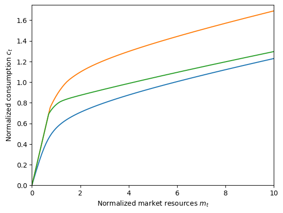
It’s not obvious from this figure, but the green consumption (with positive WealthShift) asymptotes to the blue consumption function (with zero WealthShift) as wealth becomes arbitrarily large.

Finally, recall that the wealth-in-utility model degenerates to the basic consumption-saving model when \(\WealthShare=0\). To (visually) confirm this, let’s solve a WealthUtilityConsumerType with WealthShare=0 and compare it to the basic model.

# Make and solve a wealth-in-utility consumer type that doesn't actually care about wealth
TrivialType = WealthUtilityConsumerType(cycles=0, WealthShare=0.0)
TrivialType.solve()
TrivialType.unpack("cFunc")

# Plot what should be identical consumption functions
plt.ylim(0.0, 1.75)
plt.xlabel(r"Normalized market resources $m_t$")
plt.ylabel(r"Normalized consumption $c_t$")
plot_funcs([TrivialType.cFunc[0], BaseType.cFunc[0]], 0.0, 10.0)

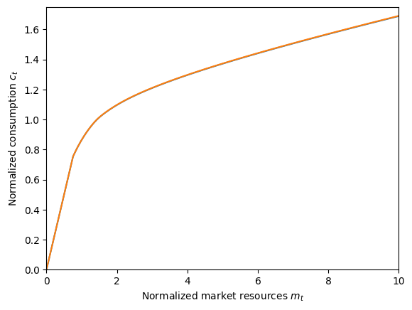
Looks the same to me!