Interactive online version:
Advanced and Uncommon HARK Concepts#
The “Gentle Introduction to HARK” and other notebooks mostly focused on the most important features that a new user would want to be familiar with. But HARK has a lot more options and deeper structure, and this notebook describes some of those “advanced” topics.
Measuring Up: Distance in HARK#
In heterogeneous agents macroeconomics, we are often interested in infinite horizon models. Such models are usually solved by “finite horizon approximation”: iteratively solving backward one period at a time until consecutive solutions are sufficiently close together that we conclude the process has converged. When using Bellman value functions, this logic relies on the fact that the Bellman operator is a contraction mapping.
The Universal Distance Metric#
But what does it mean to be “sufficiently close”? What are we even comparing when we talk about the “distance” between two candidate solutions? It depends on the context, and so HARK has a system for easily identifying “what matters” when calculating the distance between two abstract objects.
Particularly, all classes in HARK that could reasonably be part of the representation of a model solution inherit from the superclass HARK.metric.MetricObject. Essentially all this class does is provide a “universal distance metric” with simple customization.
The only thing that a subclass of MetricObject needs to specify is a class attribute called distance_criteria, which must be a list of strings. Each element of distance_criteria names an attribute of that class that should be compared if HARK is ever asked to compare two instances of that class.
HARK’s universal distance metric is nothing more than a “recursive supremum norm”. That is, it returns the highest value among element-wise distances. Its logic to compare \(A\) and \(B\) is straightforward and obvious:
if \(A\) and \(B\) are both numbers, their distance is the absolute value of their difference
if \(A\) and \(B\) are both lists, then:
if the lists have the same length, their distance is the maximum distance between corresponding elements
otherwise, the distance is the difference in their lengths
if \(A\) and \(B\) are both
numpy.array, then:if the arrays have the same shape, then the distance is the absolute value of the maximum difference between corresponding elements
if the arrays have different numbers of dimensions, return 10000 times the difference in cardinality
else return the sum of absolute differences in size in each dimension
if \(A\) and \(B\) are both dictionaries, then:
if they both have
distance_criteriaentries that match, their distance is the maximum distance among keys named in distance criteriaelse if they have the same keys, their distance is the maximum distance among their entries
otherwise, their distance is 1000, a large number
if \(A\) and \(B\) are objects of the same class, and neither is a lambda function, then their distance is given by their
distancemethodotherwise, the distance is 1000 because the objects cannot be meaningfully compared
As long as you are coding with MetricObject subclasses (like the interpolators in HARK.interpolation) and standard numeric Python objects, the distance metric will always succeed in comparing objects.
Note that comparing “incomparable” objects, like arrays of different shapes, will return a somewhat arbitrary “large” number (not near zero). This is because the sole purpose of measuring “distance” in HARK is to evaluate whether two solutions are sufficiently close. The tolerance level for such operations is usually on the order of \(10^{-4}\) to \(10^{-8}\), not \(10\) or \(1000\). Thus those “error code distances” mostly serve to ensure that a convergence criteria will definitely not be met when the comparitors are incomparable.
The tolerance for convergence is stored in the tolerance attribute of AgentType instances. It has a default of \(10^{-6}\) but can be freely changed.
HARK only compares solutions from consecutive iterations when solving an infinite horizon model. In the future, we might add extended options to (say) compare a new solution to the one \(N\) periods prior.
Getting a Description of the Distance Metric#
We’re not going to sugarcoat it: solution objects in HARK can be very complicated, with several layers of nesting. The objects that are actually being numerically compared by the distance metric might be three to six layers deep, buried in attributes, lists, and/or dictionaries.
To make it a little bit easier to understand what’s actually being compared, MetricObject (and its many descendant classes) have a describe_distance method that produces a nested description of how an object’s distance metric would be computed. Let’s see a quick example:
[1]:
from HARK.models import IndShockConsumerType

MyType = IndShockConsumerType()  # default parameters, only one non-terminal period
MyType.solve()
MyType.solution[0].describe_distance()
(ConsumerSolution): largest distance among these attributes:
  - vPfunc (MargValueFuncCRRA): largest distance among these attributes:
    - cFunc (LowerEnvelope): largest distance among these attributes:
      - functions (list) largest distance among:
        - [0] (LinearInterp): largest distance among these attributes:
          - x_list (array(49,)): greatest absolute difference among elements
          - y_list (array(49,)): greatest absolute difference among elements
        - [1] (LinearInterp): largest distance among these attributes:
          - x_list (array(2,)): greatest absolute difference among elements
          - y_list (array(2,)): greatest absolute difference among elements
    - CRRA (scalar): absolute difference of values
First, notice that the distance metric wasn’t actually used in this case– it’s a finite horizon model with only one non-terminal period! The describe_distance method is independent of distance_metric, and simply produces what would be done if the object were compared to itself.
By default, describe_distance prints its description to screen; if you would rather have it returned as a string, pass the argument display=False.
The first line indicates that the solution itself has a distance metric that depends only on its vPfunc attribute, the only item at the first level of indentation. The marginal value function vPfunc has distance criteria of cFunc (the pseudo-inverse marginal value function, which is the same thing as the consumption function) and risk aversion CRRA (very last line).
Why would CRRA be compared if it never changes during the model? Because we want distance_metric to properly compare two objects to see if they’re the same (or close to the same), and generically two marginal value functions would be different functions if they had the same pseudo-inverse marginal value function but different values of \(\rho\).
The upshot is that for an IndShockConsumerType, convergence of the solution depends on the consumption function, which is what you probably guessed in the first place. But what does that actually mean numerically?
The consumption function in this model is an instance of LowerEnvelope, an interpolation wrapper class that evaluates to the lowest function value (pointwise). The two component functions are the unconstrained consumption function (if the artificial borrowing constraint were not imposed that period) and the borrowing constraint itself; whenever the unconstrained consumption function would exceed the constraint, the agent actually consumes on the constraint.
Each of those component functions (indexed by 0 and 1) is an instance of LinearInterp, and the distance_metric compares their interpoling grid and function values– the x_list and y_list arrays.
In some cases, the output from describe_distance is so large that it’s difficult to read. To handle this, you can specify a max_depth to indicate how many layers deep the description should go. For example, we can suppress the description of the consumption function like so:
[2]:
MyType.solution[0].describe_distance(max_depth=2)
(ConsumerSolution): largest distance among these attributes:
  - vPfunc (MargValueFuncCRRA): largest distance among these attributes:
    - cFunc (LowerEnvelope): largest distance among these attributes:
      SUPPRESSED OUTPUT
    - CRRA (scalar): absolute difference of values
Uncommon Options When Solving Models#
The solve() method is usually called without any arguments, but there are a few options you can specify.
Tell Me More, Tell Me More: verbose#
First, passing verbose=True (or just True, because it is the first argument) when solving an infinite horizon model (cycles=0) will print solution progress to screen. This can be useful when developing a new model, if you want to know how long iterations take and how the solver is doing with respect to convergence.
[3]:
VerboseType = IndShockConsumerType(cycles=0)
VerboseType.solve(True)
Finished cycle #1 in 0.0 seconds, solution distance = 100.0
Finished cycle #2 in 0.0020132064819335938 seconds, solution distance = 10.088015890333434
Finished cycle #3 in 0.0009868144989013672 seconds, solution distance = 3.3534114736589693
Finished cycle #4 in 0.0010135173797607422 seconds, solution distance = 1.6699529613894306
Finished cycle #5 in 0.0009999275207519531 seconds, solution distance = 0.9967360674688486
Finished cycle #6 in 0.0010001659393310547 seconds, solution distance = 0.6602619046109499
Finished cycle #7 in 0.0010004043579101562 seconds, solution distance = 0.4680948423143789
Finished cycle #8 in 0.0 seconds, solution distance = 0.34807706501006663
Finished cycle #9 in 0.0010013580322265625 seconds, solution distance = 0.2681341538834978
Finished cycle #10 in 0.0009989738464355469 seconds, solution distance = 0.21223248168627507
Finished cycle #11 in 0.0010001659393310547 seconds, solution distance = 0.17162798586899441
Finished cycle #12 in 0.0010004043579101562 seconds, solution distance = 0.14121714401876462
Finished cycle #13 in 0.0010001659393310547 seconds, solution distance = 0.11786112023934692
Finished cycle #14 in 0.0010013580322265625 seconds, solution distance = 0.09954374358267515
Finished cycle #15 in 0.0009989738464355469 seconds, solution distance = 0.08492077965589839
Finished cycle #16 in 0.0010004043579101562 seconds, solution distance = 0.07306820983636841
Finished cycle #17 in 0.0010001659393310547 seconds, solution distance = 0.06333371450893921
Finished cycle #18 in 0.0010001659393310547 seconds, solution distance = 0.055246317280595036
Finished cycle #19 in 0.0 seconds, solution distance = 0.04845886926538645
Finished cycle #20 in 0.0010004043579101562 seconds, solution distance = 0.04271110960013802
Finished cycle #21 in 0.0010001659393310547 seconds, solution distance = 0.03780486582230225
Finished cycle #22 in 0.0010001659393310547 seconds, solution distance = 0.03358704056809492
Finished cycle #23 in 0.001001596450805664 seconds, solution distance = 0.02993783577570497
Finished cycle #24 in 0.0009987354278564453 seconds, solution distance = 0.026762425833982917
Finished cycle #25 in 0.0010001659393310547 seconds, solution distance = 0.02398495974448922
Finished cycle #26 in 0.0010030269622802734 seconds, solution distance = 0.02154418103929423
Finished cycle #27 in 0.000997781753540039 seconds, solution distance = 0.019390181762538816
Finished cycle #28 in 0.0 seconds, solution distance = 0.017481967390489572
Finished cycle #29 in 0.0010025501251220703 seconds, solution distance = 0.015785611379662612
Finished cycle #30 in 0.000997781753540039 seconds, solution distance = 0.014272839895086431
Finished cycle #31 in 0.0010001659393310547 seconds, solution distance = 0.012919936192925974
Finished cycle #32 in 0.0010001659393310547 seconds, solution distance = 0.011706884785618321
Finished cycle #33 in 0.0010001659393310547 seconds, solution distance = 0.010616703056520294
Finished cycle #34 in 0.0010001659393310547 seconds, solution distance = 0.009634898474986997
Finished cycle #35 in 0.0009877681732177734 seconds, solution distance = 0.008749044420678587
Finished cycle #36 in 0.001013040542602539 seconds, solution distance = 0.007948413988064118
Finished cycle #37 in 0.0 seconds, solution distance = 0.007223724470822646
Finished cycle #38 in 0.0010027885437011719 seconds, solution distance = 0.006566906564932307
Finished cycle #39 in 0.0009984970092773438 seconds, solution distance = 0.005970916077072452
Finished cycle #40 in 0.0009992122650146484 seconds, solution distance = 0.005429579002498741
Finished cycle #41 in 0.0010025501251220703 seconds, solution distance = 0.004937463273915199
Finished cycle #42 in 0.0009989738464355469 seconds, solution distance = 0.004489772052600927
Finished cycle #43 in 0.0010001659393310547 seconds, solution distance = 0.00408225454644251
Finished cycle #44 in 0.0 seconds, solution distance = 0.0037111311701636396
Finished cycle #45 in 0.00099945068359375 seconds, solution distance = 0.003373030500464669
Finished cycle #46 in 0.0010001659393310547 seconds, solution distance = 0.0030649359736796278
Finished cycle #47 in 0.0010023117065429688 seconds, solution distance = 0.0027841406665807256
Finished cycle #48 in 0.0009989738464355469 seconds, solution distance = 0.0025282088157077
Finished cycle #49 in 0.0009992122650146484 seconds, solution distance = 0.0022949429754119954
Finished cycle #50 in 0.0010001659393310547 seconds, solution distance = 0.0020823559119378388
Finished cycle #51 in 0.001001596450805664 seconds, solution distance = 0.0018886464739757969
Finished cycle #52 in 0.0 seconds, solution distance = 0.0017121788176552855
Finished cycle #53 in 0.0010013580322265625 seconds, solution distance = 0.0015514644867233862
Finished cycle #54 in 0.0009989738464355469 seconds, solution distance = 0.0014051468883913287
Finished cycle #55 in 0.0010001659393310547 seconds, solution distance = 0.0012719878080478253
Finished cycle #56 in 0.0010001659393310547 seconds, solution distance = 0.0011508556554602478
Finished cycle #57 in 0.0010001659393310547 seconds, solution distance = 0.0010407151830378325
Finished cycle #58 in 0.0010004043579101562 seconds, solution distance = 0.0009406184572169352
Finished cycle #59 in 0.0009999275207519531 seconds, solution distance = 0.0008496968979514463
Finished cycle #60 in 0.0 seconds, solution distance = 0.000767154229857514
Finished cycle #61 in 0.0010001659393310547 seconds, solution distance = 0.0006922602130678968
Finished cycle #62 in 0.0010018348693847656 seconds, solution distance = 0.000624345042195884
Finished cycle #63 in 0.0010001659393310547 seconds, solution distance = 0.0005627943195669616
Finished cycle #64 in 0.0009989738464355469 seconds, solution distance = 0.0005070445234864884
Finished cycle #65 in 0.0010001659393310547 seconds, solution distance = 0.0004565789051689251
Finished cycle #66 in 0.0 seconds, solution distance = 0.0004109237583840297
Finished cycle #67 in 0.0010018348693847656 seconds, solution distance = 0.00036964501506320246
Finished cycle #68 in 0.0009984970092773438 seconds, solution distance = 0.00033234512761959323
Finished cycle #69 in 0.0009996891021728516 seconds, solution distance = 0.0002986602050079057
Finished cycle #70 in 0.0010001659393310547 seconds, solution distance = 0.0002682573749837047
Finished cycle #71 in 0.0010018348693847656 seconds, solution distance = 0.00024083234929284103
Finished cycle #72 in 0.0010001659393310547 seconds, solution distance = 0.00021610717220754694
Finished cycle #73 in 0.0009989738464355469 seconds, solution distance = 0.0001938281357389826
Finished cycle #74 in 0.001001596450805664 seconds, solution distance = 0.0001737638473713332
Finished cycle #75 in 0.0 seconds, solution distance = 0.00015570343805260123
Finished cycle #76 in 0.0009987354278564453 seconds, solution distance = 0.00013945489982702952
Finished cycle #77 in 0.001001596450805664 seconds, solution distance = 0.00012484354371933293
Finished cycle #78 in 0.0009987354278564453 seconds, solution distance = 0.00011171056964087711
Finished cycle #79 in 0.0010001659393310547 seconds, solution distance = 9.991174074386322e-05
Finished cycle #80 in 0.0010001659393310547 seconds, solution distance = 8.931615549556682e-05
Finished cycle #81 in 0.0 seconds, solution distance = 7.980511119587419e-05
Finished cycle #82 in 0.0010018348693847656 seconds, solution distance = 7.12710531196592e-05
Finished cycle #83 in 0.0009989738464355469 seconds, solution distance = 6.361660386744461e-05
Finished cycle #84 in 0.0009999275207519531 seconds, solution distance = 5.675366786039859e-05
Finished cycle #85 in 0.0010018348693847656 seconds, solution distance = 5.060260605649347e-05
Finished cycle #86 in 0.0010001659393310547 seconds, solution distance = 4.5091476412739695e-05
Finished cycle #87 in 0.0 seconds, solution distance = 4.0155335675251536e-05
Finished cycle #88 in 0.0009996891021728516 seconds, solution distance = 3.573559836667073e-05
Finished cycle #89 in 0.0010006427764892578 seconds, solution distance = 3.1779449082502964e-05
Finished cycle #90 in 0.0009984970092773438 seconds, solution distance = 2.8239304256771902e-05
Finished cycle #91 in 0.0010004043579101562 seconds, solution distance = 2.507231993220671e-05
Finished cycle #92 in 0.0010001659393310547 seconds, solution distance = 2.2239942116364375e-05
Finished cycle #93 in 0.0010004043579101562 seconds, solution distance = 1.970749654489623e-05
Finished cycle #94 in 0.0 seconds, solution distance = 1.7443814823714376e-05
Finished cycle #95 in 0.0010013580322265625 seconds, solution distance = 1.54208941594014e-05
Finished cycle #96 in 0.0010001659393310547 seconds, solution distance = 1.3613587938721139e-05
Finished cycle #97 in 0.0009989738464355469 seconds, solution distance = 1.1999324726730265e-05
Finished cycle #98 in 0.0010001659393310547 seconds, solution distance = 1.0557853295622976e-05
Finished cycle #99 in 0.0 seconds, solution distance = 9.271011538913854e-06
Finished cycle #100 in 0.0010001659393310547 seconds, solution distance = 8.122517190400913e-06
Finished cycle #101 in 0.0010004043579101562 seconds, solution distance = 7.097778525810838e-06
Finished cycle #102 in 0.0010004043579101562 seconds, solution distance = 6.183723237906946e-06
Finished cycle #103 in 0.0010001659393310547 seconds, solution distance = 5.368643900993675e-06
Finished cycle #104 in 0.0010001659393310547 seconds, solution distance = 4.642058520687442e-06
Finished cycle #105 in 0.0010020732879638672 seconds, solution distance = 3.99458479938275e-06
Finished cycle #106 in 0.0 seconds, solution distance = 3.4178268535356437e-06
Finished cycle #107 in 0.0009987354278564453 seconds, solution distance = 2.9042732059281207e-06
Finished cycle #108 in 0.0009868144989013672 seconds, solution distance = 2.4472050079715757e-06
Finished cycle #109 in 0.0010151863098144531 seconds, solution distance = 2.0406135377015744e-06
Finished cycle #110 in 0.0009999275207519531 seconds, solution distance = 1.679126009790366e-06
Finished cycle #111 in 0.0009987354278564453 seconds, solution distance = 1.357939007018416e-06
Finished cycle #112 in 0.0010018348693847656 seconds, solution distance = 1.0727586712278026e-06
Finished cycle #113 in 0.0 seconds, solution distance = 8.19747068891985e-07
Notice that the solver terminated as soon as the distance went below \(10^{-6}\), the default value for tolerance.
Turning Off pre_solve and post_solve#
When solve() is invoked, the AgentType instance usually runs their pre_solve() method before jumping into the main solver loop over periods. In some situations, the user might want to skip the call to pre_solve()– maybe it would undo some unusual work that the user wants in place. To do so, simply pass presolve=False in the call to solve().
Likewise, after the solution loop has completed its work, just before exiting the call to solve(), HARK runs the post_solve() method for that AgentType subclass. In the unusual situation in which a user does not want that method run, just pass postsolve=False to solve().
Take It From the Middle: from_solution and from_t#
HARK’s default behavior is to solve all model periods, starting from solution_terminal and working back to the very first period. A user can override this with two interrelated options.
In case of some custom terminal solution (or continuation solution), the solution object can be passed in the from_solution argument. One use case for this is solving an infinite horizon model by starting from the solution to a “nearby” model, rather than from the proper terminal period.
Likewise, the from_t optional argument can be used to indicate which time index to actually start the solver from. This option is only compatible with cycles=1. In conjunction with from_solution, this can be used to (say) impose some terminal solution in the middle of the life-cycle, and only solve the problem from that point backward. That terminal solution might be the first period of some other model for a “later phase” of life.
If you pass an argument for from_t but not from_solution, then HARK will use solution_terminal as the succeeding solution when trying to solve the one-period problem at time index from_t.
Utility Functions#
Utility functions and related objects can be imported from HARK.rewards. These functions used to be in HARK.utilities, but we decided that it was too confusing to have both “utility functions” and “utility tools” in the same file.
Almost all consumption-saving models in HARK use constant absolute risk aversion (CRRA) utility functions over consumption. There are two main ways to use CRRA utility from HARK.rewards.
In-Line Utility Functions#
First, there are individual functions like CRRAutility and CRRAutilityP that take in a (possibly vector-valued) consumption argument and a CRRA coefficient. They do exactly what you’d expect, and are programmed to correctly handle \(\rho=1\) being log utility.
In most circumstances, it’s convenient to locally define the (marginal) utility function for the currently relevant value of \(\rho\).
[4]:
from HARK.rewards import CRRAutility, CRRAutilityP, UtilityFuncCRRA
import matplotlib.pyplot as plt
from HARK.utilities import plot_funcs
[5]:
rho = 2.5  # maybe this parameter was passed from elsewhere
u = lambda x: CRRAutility(x, rho)
uP = lambda x: CRRAutilityP(x, rho)
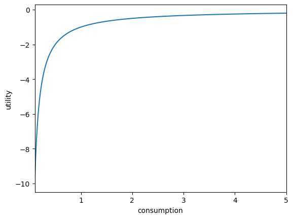
[6]:
plt.xlabel("consumption")
plt.ylabel("utility")
plot_funcs(u, 0.1, 5.0)
plt.xlabel("consumption")
plt.ylabel("marginal utility")
plot_funcs(uP, 0.1, 5)

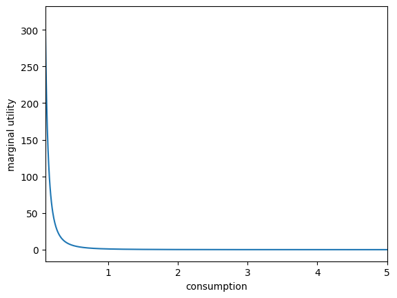
As a notational convention, HARK uses a capital P to denote “prime”, and _inv for “inverse”. HARK.rewards defines several layers of derivative and inverses for CRRA utility:
CRRAutility: utility functionCRRAutilityP: marginal utility functionCRRAutilityPP: marginal marginal utility functionCRRAutilityPPP: marginal marginal marginal utility functionCRRAutilityPPPP: marginal marginal marginal marginal utility functionCRRAutility_inv: inverse utility functionCRRAutilityP_inv: inverse marginal utility functionCRRAutility_invP: marginal inverse utility functionCRRAutilityP_invP: marginal inverse marginal utility function
Utility Function Structure#
The second way to use CRRA utility is to simply import the class UtilityFuncCRRA and instantiate it with a single argument for \(\rho\). This object then represents the utility function and all of its derivatives and inverses. Let’s see an example.
[7]:
U = UtilityFuncCRRA(2.0) # CRRA utility function with rho=2
[8]:
plt.xlabel("consumption")
plt.ylabel("utility")
plot_funcs(U, 0.1, 5.0) # treat it like a function
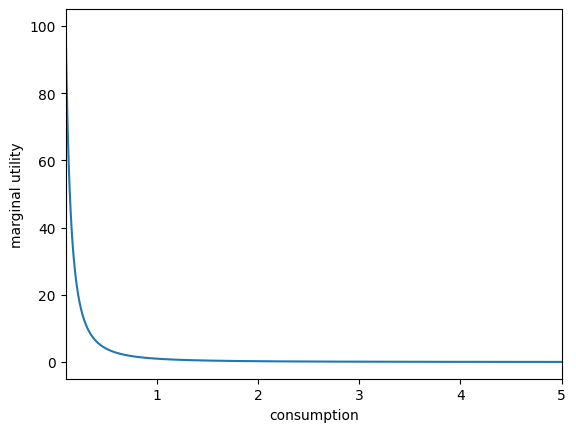
plt.xlabel("consumption")
plt.ylabel("marginal utility")
plot_funcs(U.derivative, 0.1, 5) # use its derivative method for marginal utility
plt.xlabel("utility")
plt.ylabel("consumption")
plot_funcs(U.inverse, -10.0, -0.1) # use its inverse method
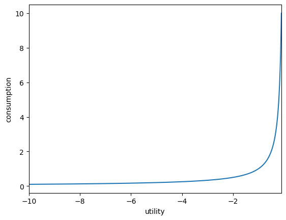
The derivative method accepts a second optional argument of order with a default of 1, indicating the order of the derivative (first to fourth order).
The inverse method also accepts an order argument as an ordered pair (0,0) to (1,1). For a simple mnemonic, order refers to the number of Ps in the function CRRAutility[#1]_inv[#2]. The default is (0,0), which is just the inverse of utility.
Other Utility Functions in HARK.rewards#
Four other utility functions have various levels of support in HARK, but are rarely used:
Stone-Geary: Modified CRRA utility of the form \(U(c) = b \frac{(c+a)^{1-\rho}}{1-\rho}\), with a default of \(b=1\).
Constant Absolute Risk Aversion (CARA): Normalized exponential utility of the form \(U(c) = 1 - \exp(-\alpha c) / \alpha\).
Cobb-Douglas: Cobb-Douglas aggregator for an aribtrary number of goods: \(U(x) = \prod_{j=1}^J x_j^{\zeta_j}\).
Constant Elastisticity of Substitution (CES): CES aggregator characterized by elasticity \(\epsilon\), shares \(\zeta\), scaling factor \(\alpha\) and homogeneity degree \(\eta\): \(U(x) = \alpha \left(\prod_{j=1}^J \zeta_j x_j^\epsilon \right)^{\eta / \epsilon}\).
Each of these utility forms has a utility function class, but the inverse methods are not defined for multiple-input forms.
Representing Distributions#
The HARK.distributions module provides a fairly wide array of representations of distributions for random variables.
Basics of Distributions in HARK#
All distribution classes have some common methods and attributes:
seed: An integer attribute that can be set at instantiation. It is used as the seed for the distribution’s internal random number generator.random_seed(): A method to draw a new random seed for the distribution. This is not recommended for computations that need to be precisely replicated.reset(): A method to reset the distribution’s internal RNG by using its own storedseed.draw(N): A method to generate \(N\) random draws from the distribution.discretize(N, method): A method to generate aDiscreteDistributionbased on this distribution object. The only universally required input is \(N\), the number of nodes in the discretization, but a stringmethodcan be passed as well, along with method-specifickwds.infimum: The greatest lower bound for the support of the distribution; it is always an array, even for univariate distributions.supremum: The least upper bound for the support of the distribution; it is always an array.
Our Workhorse: DiscreteDistribution#
Almost all computation in HARK actually uses discretized approximations of continuous RVs. The default discretization method is equiprobable (which actually has options for non-equiprobable discretizations in some cases), rather than Gaussian methods. This approach is meant to ensure that the mean of the distribution is exactly preserved by the discretization.
The key attributes of a DiscreteDistribution are pmv and atoms. The pmv is the probability mass vector, a np.array that should sum to 1, representing the probability masses for each of the nodes.
The discretized nodes are stored in the atoms attribute as a 2D np.array, even for univariate distributions. The first dimension (axis=0) indexes multiple components of a multivariate distribution, and the second dimension (axis=1) index the nodes.
A DiscreteDistribution that is created from a continuous distribution object using its discretize method should have an attribute called limit with information about how it was generated:
dist: a reference to the continuous distribution itselfmethod: the name of the method that was used to build the approximationN: the number of nodes requestedinfimum: the infimum of the continuous distribution from which it was madesupremum: the supremum of the continuous distribution from which it was made
We included this so that HARK’s solvers can use (particularly) information about the “best” and “worst” things that can happen, even if they don’t appear in the discretization. This is sometimes important for bounding behavior of the model solution.
Say My Name: DiscreteDistributionLabeled#
The default behavior in HARK is for multivariate distributions to simply be indexed by number. E.g. a joint distribution of permanent and transitory income shocks might have \(\psi\) at index 0 and \(\theta\) at index 1. However, we also have an extended class called DiscreteDistributionLabeled that allows more information to be provided.
The additional fields for a Labeled distribution are (all optional):
name: a name or title for the distribution, for describing its purposeattrs: a dictionary of attributes, for arbitrary usevar_names: a list of strings naming each variable in the distributionvar_attrs: a list of dictionaries with attributes for each variable in the distribution
A DiscreteDistributionLabeled can be instantiated in two ways:
Passing a
pmv,atoms, andseedalong with any of the optional arguments, generating a completely new object.Passing a
DiscreteDistributionalong with any optional arguments, effectively “converting” the input distribution.
Example Usage#
We won’t show everything in HARK.distribution here, but this is a sampling (no pun intended) of some key features.
[9]:
import numpy as np
from HARK.distributions import (
    Lognormal,
    add_discrete_outcome,
    add_discrete_outcome_constant_mean,
    DiscreteDistributionLabeled,
    expected,
)
[10]:
# Make a lognormal distribution and draw twenty numbers from it
F = Lognormal(mu=0.2, sigma=0.7, seed=10202025)
print(F.draw(20))
[0.88164369 1.27060758 0.82340037 0.32759431 1.57918536 1.23739098
 1.52478804 2.82758116 1.77216365 0.45260362 1.03188809 0.77631269
 4.06323317 0.97823279 2.11448412 2.90854828 0.89516082 2.9296455
 0.8560163  0.75149165]
[11]:
# Make a discrete approximation of the lognormal and print information about it
F_approx = F.discretize(N=9)
print(F_approx.pmv)  # equiprobable!
print(F_approx.atoms)  # univariate, but is a 2D array
print(np.dot(F_approx.atoms, F_approx.pmv))  # mean of discretization
print("Mean of true distribution is " + str(np.exp(F.mu + 0.5 * F.sigma**2)))
[0.11111111 0.11111111 0.11111111 0.11111111 0.11111111 0.11111111
 0.11111111 0.11111111 0.11111111]
[[0.38465583 0.61952063 0.80874565 1.0034799  1.2233456  1.49178328
  1.85298459 2.4281933  4.231703  ]]
[1.5604902]
Mean of true distribution is 1.5604901958326667
[12]:
# Draw twenty numbers from the discretization
F_approx.draw(20)
[12]:
array([2.4281933 , 0.38465583, 0.80874565, 0.61952063, 4.231703  ,
       0.61952063, 0.61952063, 2.4281933 , 1.49178328, 1.2233456 ,
       1.49178328, 1.0034799 , 2.4281933 , 1.85298459, 1.49178328,
       2.4281933 , 1.0034799 , 1.0034799 , 0.80874565, 0.61952063])
Notice that when drawing from the true distribution F, we got values from its entire support (any positive real), but when drawing from the 9 point equiprobable discretization, we can only get 9 different values.
[13]:
# Add a point mass at zero
G = add_discrete_outcome(F_approx, x=0.0, p=0.1)
print(G.pmv)  # other probabilities proportionally scaled down
print(G.atoms)
print(np.dot(G.atoms, G.pmv))
[0.1 0.1 0.1 0.1 0.1 0.1 0.1 0.1 0.1 0.1]
[[0.         0.38465583 0.61952063 0.80874565 1.0034799  1.2233456
  1.49178328 1.85298459 2.4281933  4.231703  ]]
[1.40444118]
[14]:
# Add a point mass at zero, but preserve the original mean
H = add_discrete_outcome_constant_mean(F_approx, x=0.0, p=0.1)
print(H.pmv)
print(H.atoms)
print(np.dot(H.atoms, H.pmv))
[0.1 0.1 0.1 0.1 0.1 0.1 0.1 0.1 0.1 0.1]
[[0.         0.42739536 0.68835626 0.89860627 1.11497766 1.35927289
  1.65753698 2.05887176 2.69799255 4.70189222]]
[1.5604902]
[15]:
# Make a labeled version of that distribution
H_labeled = DiscreteDistributionLabeled.from_unlabeled(
    H, name="permanent income shocks", var_names=["PermShk"]
)
[16]:
# Calculate the expectation of a function of our random variable
temp_func = lambda x, y: x["PermShk"] ** 2 + y
expected_value = expected(temp_func, H_labeled, args=(3.0,))
print(expected_value)
7.092812838769875
The expected utility is useful for writing shorter code within our solvers. It can be used with both ordinary DiscreteDistributions and with Labeled ones. The function passed to expected as its first argument should always take a distribution as its first argument, and index by number or name. Additional arguments are provided in order as args.
Estimation and Optimization#
HARK doesn’t provide many tools for estimating the parameters of particular models– our take is that the details of each particular application are too bespoke to provide a meaningful interface for estimation. We do have a HARK.estimation module, but it is mostly a remapping of functions from scipy.optimize.
In particular, the functions minimize_nelder_mead and minimize_powell remap scipy.optimize.fmin and scipy.optimize.fmin_powell, with a few additional options. In particular, the former function permits an optional argument of which_vars as a Boolean array with length equal to the number of arguments of the function to be minimized; it indicates which dimensions should actually be optimized.
As usual for scipy.optimize functions, the minimand should accept a single input vector. That is, if there are 5 arguments to the function to be minimized, they should be passed as a single np.array.
HARK does provide one hand-programmed optimizer: a parallelized Nelder-Mead minimizer, adapted from Lee and Wiswall. This uses “embarrassingly parallel” techniques from joblib, literally writing to and reading from disk as it spawns and deletes new Python processes. Because of this significant overhead, it should only be used for functions that are relatively “expensive” to evaluate– a few seconds, at least.
See the full documentation for parallelNelderMead for all of the options, but the key inputs are:
obj_func: The function to be optimized, with the same format as usual.guess: Starting point for the optimization, around which a simplex will be built.perturb: A vector of perturbations in each argument, used for building the simplex. Ifperturb[j]is0, that dimension is excluded from the optimization. If noperturbis provided, the default is to optimize all dimensions with an initial simplex of 10% of theguess.P: The degree of parallelization– how many nodes of the simplex to attempt to update on each iteration. Defaults to 1, which is standard Nelder-Mead.maxthreads: The largest number of Python threads to run simultaneously. This can be no greater or less thanP, which is relevant when evaluating the initial simplex or executing a shrink step.name: A filename for optionally storing progress of the search; must be used in conjuction with next two arguments. Useful for very long optimizations that might be interupted by computer downtime.resume: Whether the optimization should resume from prior saved progress (in filename) or start from scratch.savefreq: Frequency (in number of iterations) of writing progress to disk, defaulting to 1 (write after every iteration).
Parallelizing Operations#
HARK has a basic tool for parallelizing operations across AgentType instances. If you have a population of agents that has ex ante heterogeneity– they differ in their parameters, or possibly even in their model, their microeconomic problems can be solved independently and simultaneously. If there is no macroeconomic interaction among AgentType instances, then their models can be simulated independently as well.
The relevant function is HARK.parallel.multi_thread_commands, which takes three arguments:
agent_list: a list ofAgentTypeinstances for which parallel work should be performedcommand_list: a list of strings naming methods to be runnum_jobs: optionally, a maximum number of Python threads to spawn
The function returns no output; agent_list itself is changed by running multi_thread_commands.
There are two caveats when using multi_thread_commands:
Each element of
command_listmust include()at the end, e.g.solve(). This will be changed in the future.AgentTypeinstances can be large and thus take considerable time topicklewhen writing to disk (and then reading from disk). This is particularly the case when model is solved and simulated by the multithreaded process, as bothsolutionandhistorycan be large. If you find that this is a problem, try to find ways to “pre-process” the output at theAgentTypeinstance level, before it exits the spawned thread, and delete the attributes that you don’t strictly “need”.
We have also included a trivial multi_thread_commands_fake function, which replicates the interface of multi_thread_commands but does not use the Parallel package for spawning processes. Instead, it simply loops over the elements of agent_list and executes the methods for each one. This function is included to have a quick way to “turn off” multi-threading in your code.
Life-Cycle Parameter Calibrations#
The default parameters for each AgentType subclass are just meant to be workable examples, not represent anything “realistic”. Some of the default parameters are reasonable or vaguely in the ballpark of values you might get from empirical measurements (e.g. a CRRA of 2 or risk free interest factor of 1.02), but this is mostly coincidence or us being too lazy to make up unreasonable values.
The HARK.Calibration module includes some off-the-shelf calibrations of life-cycle processes, estimated by people who are better with data than we are. It also has some functions for making particular parametric distributions for income processes.
Income Processes#
[17]:
from HARK.Calibration.Income.IncomeTools import Cagetti_income, parse_income_spec
See the documentation for full details, but the main tool for handling life-cycle income specifications is parse_income_spec. This function takes a large number of inputs, but conveniently we have provided some dictionaries for quick use. This function produces a dictionary with a variety of income process parameters, which can be passed to an AgentType subclass to produce a realistically calibrated instance of that class (with HARK’s default income process, or something similar to
it).
[18]:
# Make an income process dictionary for high-school-educated men based on Cagetti (2003)
my_income_params = parse_income_spec(age_min=22, age_max=110, **Cagetti_income["HS"])
print(my_income_params.keys())
print(
    len(my_income_params["PermShkStd"])
)  # number of non-terminal periods in the model
dict_keys(['PermGroFacAgg', 'PermGroFac', 'PermShkStd', 'TranShkStd', 'P0', 'pLogInitMean', 'T_retire'])
88
Mortality Processes#
HARK can also construct life-cycle mortality probabilities based on Social Security Administration actuarial tables. This tool is currently buried quite deep in HARK, at HARK.Calibration.life_tables.us_ssa.SSATools.parse_ssa_life_table, but we will expose it more conveniently in the near future.
[19]:
from HARK.Calibration.life_tables.us_ssa.SSATools import parse_ssa_life_table
[20]:
# Make survival probabilities for men born in 1980
my_LivPrb = parse_ssa_life_table(age_min=22, age_max=110, female=False, cohort=1980)
print(len(my_LivPrb))
print(my_LivPrb[:10])  # first 10 survival probabilities, from start of model life
88
[0.998541, 0.998511, 0.998545, 0.99852, 0.998489, 0.998549, 0.998583, 0.998606, 0.998592, 0.998535]
Unlike parse_income_spec, this function returns only survival probabilities, which are used as LivPrb in most HARK models.
Using Parsed Parameters in a Model#
Let’s show a simple example of how to use the parameters we imported in an AgentType instance.
[21]:
# Put the parsed parameters together into an IndShockConsumerType
T = 110 - 22  # number of non-terminal periods
CalibratedType = IndShockConsumerType(
    LivPrb=my_LivPrb,
    T_cycle=T,
    Rfree=T * [1.02],
    **my_income_params,
)
[22]:
# Solve the life-cycle problem for this agent
CalibratedType.solve()
[23]:
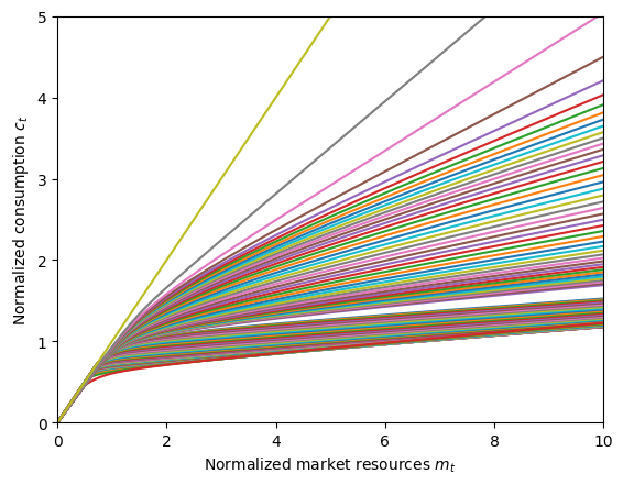
# Plot the consumption function at all ages
CalibratedType.unpack("cFunc")
plt.xlabel(r"Normalized market resources $m_t$")
plt.ylabel(r"Normalized consumption $c_t$")
plt.ylim(0.0, 5.0)
plot_funcs(CalibratedType.cFunc, 0.0, 10.0)
Quick and Dirty Function Plots#
HARK has some basic convenience functions for making simple function plots. These are mostly meant to be used in live/interactive sessions when you’re exploring your model, not to produce perfectly formatted figures for publication. We have provided very limited formatting options, and no option to save anyway.
Basic 1D Plotting: plot_funcs#
Throughout this notebook and others, you’ve probably noticed us using plot_funcs, which is used for plotting one or more real functions with simple syntax: plot_funcs(your_function(s), bottom, top). Note that your_function(s) can be a single function or a list of functions.
You can pre-format the figure with matplotlib instructions before calling plot_funcs. In this notebook, we sometimes set the ylim, xlabel, and ylabel. The arguments xlabel, ylabel, and legend_kwds can also optionally be passed to plot_funcs.
Plotting “Slices” of Functions with Multiple Arguments#
Many functions produced by HARK have more than one argument, such as when there is more than one continuous state variable. HARK includes a simple function for quickly plotting cross-sections or “slices” of such functions with plot_func_slices.
The key concepts for plot_func_slices are the xdim and zdim, representing the \(x\) plotting dimension (the function argument that is continuously varied along the horizontal axis) and the discretized \(z\) dimension (the function argument that takes on a different value for each slice). Both of these are index numbers referencing the argument number for the function to be plotted; by default, xdim=0 and zdim=1.
The syntax for plot_func_slices is somewhat more complex than for plot_funcs. In addition to passing the function itself and the lower and upper bounds on \(x\), you must also specify which values of \(z\) should be plotted. This can be done in two ways:
Pass arguments called
zminandzmaxto specify the lower and upper bounds of \(z\). By default, a grid with 11 linearly spaced points will be used, but this can be changed with the argumentsznandzorder.Pass an argument called
Zas a list (or array) of user-specified \(z\) values.
You must choose exactly one of these methods; passing neither or both will result in an error.
Let’s use the consumption function for PrefShockConsumerType as an example, first importing what we need.
[24]:
from HARK.models import PrefShockConsumerType
from HARK.utilities import plot_func_slices

PrefType = PrefShockConsumerType(cycles=0)
PrefType.solve()
PrefType.unpack("cFunc")  # make solution[t].cFunc available as cFunc[t] for convenience
[25]:
plot_func_slices(
    PrefType.cFunc[0],
    0.0,
    5.0,
    zmin=0.35,
    zmax=2.7,
    xlabel=r"Normalized market resources $m_t$",
    ylabel=r"Normalized consumption $c_t$",
)
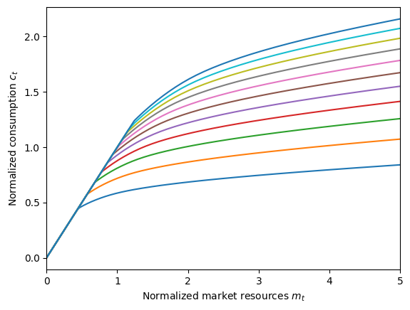
Each one of those plots represents the consumption function when holding fixed preference shock \(\eta\) at some level of interest (for values between 0.35 and 2.7). We could instead plot consumption with respect to \(\eta\) while holding \(m_t\) fixed by specifying xdim and zdim.
[26]:
plot_func_slices(
    PrefType.cFunc[0],
    0.35,
    2.7,
    xdim=1,
    zdim=0,
    zmin=0.1,
    zmax=5.0,
    zn=26,
    xlabel=r"Preference shock $\eta_t$",
    ylabel=r"Normalized consumption $c_t$",
)
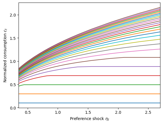
Notice here that for low market resource levels (the blue, orange, and green plots near the bottom), the consumption function is flat with respect to \(\eta\). That represents the liquidity constrained portion of the consumption function where the agent is already spending as much as they can. Increasing their preference for consumption makes them want to consume more, but they don’t actually consume more. At somewhat higher values of \(m_t\), they have high enough market resources that they are unconstrained for low \(\eta\) but become constrained for higher \(\eta\). At sufficiently high \(m_t\), the consumer is not liquidity constrained for any \(\eta\) plotted here.
Finding “Target” or Steady-State Values#
Most HARK AgentType subclasses now have a method to automatically calculate the “target” level of an endogenous state variable, using the find_target method. The target level of a state \(x\) satisfies \(\mathbb{E}[ \Delta x ] = 0\), so that an agent currently at \(x_t\) expects to be at the same value (on average) in \(t+1\) if they survive. Moreover, a target level must be locally stable, so that at values of \(x_t\) below the target, the agent expects
\(\mathbb{E}[ \Delta x ] > 0\) and for \(x_t\) above the target, they expect the state to fall.
Basic Usage for find_target#
The basic syntax is straightforward in many cases: the user simply names the variable they want to find the target for, e.g. MyType.find_target("mNrm"). (Recall from the simulation introduction that you can view a list of model variable names with MyType.describe_model().) Let’s first do a quick example with the workhorse IndShockConsumerType:
[27]:
MyType = IndShockConsumerType(cycles=0)  # default parameters, infinite horizon
MyType.solve()  # need to solve the model in order to find target or steady state
m_targ = MyType.find_target("mNrm")
print("Found target market resources ratio of {:.6f}".format(m_targ))
Found target market resources ratio of 1.492786
Because it’s the canonical workhorse model in HARK, IndShockConsumerType already had a “handwritten” method for finding target market resources, long before we added the generic method. As a quick test, let’s compare that “hand calculated” value to the one from the general method:
[28]:
m_targ_old = MyType.bilt["mNrmTrg"]
print(
    "The hand-coded method found a target market resources ratio of {:.6f}".format(
        m_targ_old
    )
)
The hand-coded method found a target market resources ratio of 1.492786
Note that the find_target method has some limitations:
It only works on standard infinite horizon models:
cycles=0andT_cycle=1.It can currently only solve for one endogenous state variable at a time; this excludes
BasicHealthConsumerType.
Providing Additional Required Information#
HARK has several models with one or more exogenous state variables, e.g. the persistent income level pLvl for PersistentShockConsumerType or the preference shock PrefShk for the PrefShockConsumerType. For those types, pLvl and PrefShk must respectively be known at the time the consumption decision is made. For find_target to work, the user needs to also pass the steady-state value of the exogenous state variable(s) as keyword arguments. In all current HARK models,
the steady state of such variables should be obvious to the user based on the parameters.
For example, the default parameters for PersistentShockConsumerType have agents being “born” with an average pLvl of \(1\), and then they experience mean one persistent income shocks with no growth trend. It should be pretty obvious that the “steady state” value of pLvl is \(1\).
[29]:
from HARK.models import PersistentShockConsumerType

PersistentType = PersistentShockConsumerType(cycles=0)
PersistentType.solve()
m_targ_prst = PersistentType.find_target("mLvl", pLvl=1.0)
print(
    "The default persistent shock consumer type has target market resources level of {:.6f}".format(
        m_targ_prst
    )
)
The default persistent shock consumer type has target market resources level of 1.730613
As a second example, the default parameters for a PrefShockConsumerType involve a mean one preference shock distribution, so target market resources can be found with:
[30]:
from HARK.models import PrefShockConsumerType

PrefShockType = PrefShockConsumerType(cycles=0)
PrefShockType.solve()
m_targ_pref = PrefShockType.find_target("mNrm", PrefShk=1.0)
print(
    "The default preference shock consumer type has target market resources level of {:.6f}".format(
        m_targ_pref
    )
)
The default preference shock consumer type has target market resources level of 1.525104
Common Failure Modes for find_target#
The target level of a state variable does not always exist. When find_target fails to find any target level, it returns np.nan. Note that this can occur for several reasons:
There really is no target value anywhere.
There is a target value, but it is outside of the search bounds; by default, \(x \in [0,100]\) but can be changed with argument
bounds.There is a target value, but additional state information needed to be passed to
find_target.
Let’s see an example for each of these failure modes. First, the agent might be so patient that (even though their policy function is well defined), they always want to accumulate more wealth, and there is simply no target anywhere.
[31]:
PatientType = IndShockConsumerType(cycles=0, DiscFac=1.0)
PatientType.solve()
print(PatientType.bilt["mNrmTrg"])
print(PatientType.find_target("mNrm"))
nan
nan
Second, the target value exists, but is outside the default bounds. To make this happen, we’ll construct a consumer who has no artificial borrowing constraint and never faces a low-income “unemployment” shock. The lower bound of their mNrm state space goes to a significantly negative level, and the target \(m_t\) is below zero, outside of the default search region.
[32]:
UnboundType = IndShockConsumerType(cycles=0, UnempPrb=0.0, BoroCnstArt=None)
UnboundType.solve()
print(UnboundType.bilt["mNrmTrg"])
print(UnboundType.find_target("mNrm"))
-1.7250338547911441
nan
To fix this, let’s get the lower boundary of mNrm and use that as the lower bound of the search.
[33]:
mNrmMin = UnboundType.solution[0].mNrmMin
print(UnboundType.find_target("mNrm", bounds=[mNrmMin, 100.0]))
-1.7250338508597622
The third failure mode is an error by the user in providing sufficient information. Suppose you wanted to know steady state bNrm, bank balances before receiving labor income yNrm. Because transitory income shocks are mean one in the default parameters, and yNrm=TranShk, we should expect that target bNrm is exactly one less than target mNrm. But if we just ask find_target for target bNrm, it will fail:
[34]:
print(MyType.find_target("bNrm"))
nan
What happened here? To understand, we need to look at how the agent’s model is written out:
[35]:
MyType.describe_model()
ConsIndShock: Consumption-saving model with permanent and transitory income shocks and a risk-free asset.

----------------------------------
%%%%%%%%%%%%% SYMBOLS %%%%%%%%%%%%
----------------------------------
kNrm (float)        : beginning of period capital, normalized by p_{t-1}
pLvlPrev (float)    : inbound permanent income level, before growth
yNrm (float)        : normalized labor income
pLvl (float)        : permanent income level
bNrm (float)        : normalized bank balances
mNrm (float)        : normalized market resources
cNrm (float)        : normalized consumption
aNrm (float)        : normalized end-of-period assets
live (bool)         : whether the agent survives
Rfree (param)       : risk free return factor on assets
PermGroFac (param)  : expected permanent income growth factor
LivPrb (param)      : survival probability at end of period
cFunc (func)        : consumption function over market resources
IncShkDstn (dstn)   : joint distribution of permanent and transitory shocks
pLvlInitDstn (dstn) : distribution of permanent income at model birth
kNrmInitDstn (dstn) : distribution of normalized capital holdings at birth
PermShk (float)     :
TranShk (float)     :
G (float)           :
dead (bool)         : whether agent died this period
t_seq (int)         : which period of the sequence the agent is on
t_age (int)         : how many periods the agent has already lived for
----------------------------------
%%%%% INITIALIZATION AT BIRTH %%%%
----------------------------------
pLvlPrev ~ pLvlInitDstn : draw initial permanent income from distribution
kNrm ~ kNrmInitDstn     : draw initial capital from distribution
----------------------------------
%%%% DYNAMICS WITHIN PERIOD t %%%%
----------------------------------
(PermShk,TranShk) ~ IncShkDstn : draw permanent and transitory income shocks
yNrm = TranShk                 : normalized income is the transitory shock
G = PermGroFac*PermShk         : calculate permanent income growth
pLvl = pLvlPrev*G              : update permanent income level
bNrm = Rfree*kNrm/G            : calculate normalized bank balances
mNrm = bNrm+yNrm               : calculate normalized market resources
cNrm = cFunc@(mNrm)            : evaluate consumption from market resources
aNrm = mNrm-cNrm               : calculate normalized end-of-period assets
live ~ {LivPrb}                : draw survival
dead = 1-live                  : dead are non-survivors
----------------------------------
%%%%%%% RELABELING / TWIST %%%%%%%
----------------------------------
aNrm[t-1] <---> kNrm[t]
pLvl[t-1] <---> pLvlPrev[t]
-----------------------------------
When find_target is asked to find target \(b_t\), it looks through the dynamics and finds where bNrm is set, then tests different values of it by starting the period at that point and looping back around to the same spot. When it does so, it uses fake / dummy values for all model variables that should have been assigned before bNrm. That includes income yNrm, so in the very next step, it calculates mNrm = bNrm + yNrm… and uses nonsense data for yNrm. It thus
fails to find a target \(b_t\) because it doesn’t have correct information about \(y_t\).
To fix this, we need to pass yNrm=1.0, the average or steady state value, to the method as well:
[36]:
print(MyType.find_target("bNrm", yNrm=1.0))
0.49278579223515967
As expected, target \(b_t\) is exactly \(1\) less than target \(m_t\) for this agent.
Guiding Principle for Additional Required Information#
In general, you should only try to calculate a target value at “informational chokepoints”: moments in the sequence of events where you know what variables will ever be referenced beyond that point. The most straightforward “informational chokepoint” is usually the decision-time state space: whatever the control variable (and Bellman value function) is conditioned on.
To make this point clear, consider the preference shock model. To get a sensible target for \(m_t\), we needed to pass the mean or steady state value of preference shock \(\eta_t\), which was known to be \(1\). However, we do not need to pass PrefShk = 1.0 if we ask for target end-of-period assets \(a_t\). At the end of the period, \(\eta_t\) has already played its role and is water under the bridge; it is not informative about the future.
[37]:
print(PrefShockType.find_target("aNrm"))
0.623920206603688
[ ]: