Interactive online version:
Advanced Examples of HA-SSJ’s#
This notebook has additional examples of the kinds of things you can do with HARK’s heterogeneous agent sequence space Jacobian (HA-SSJ) constructor functionality. If you don’t know anything at all about that, we recommend you read the HA-SSJ tutorial notebook first, or even the notebook that explains what an SSJ is.
[1]:
# First, let's import some basic things and define a plotting function
from time import time
import matplotlib.pyplot as plt
from HARK.utilities import plot_funcs
import numpy as np


# Define a simple function for plotting SSJs
def plot_SSJ(jac, S, outcome, shock, t_max=None):
    top = jac.shape[0] + 1 if t_max is None else t_max
    if type(S) is int:
        S = [S]
    for s in S:
        plt.plot(jac[:, s], "-", label="s=" + str(s))
    plt.legend()
    plt.xlabel(r"time $t$")
    plt.ylabel("rate of change of " + outcome)
    plt.title("SSJ for " + outcome + " with respect to " + shock + r" at time $s$")
    plt.tight_layout()
    plt.xlim(-1, top)
    plt.show()
Using Alternative Constructors#
Each AgentType subclass is specified to work “off the shelf”, with default constructors that build complex model objects (like the distribution of income shocks) from primitive parameters. But what if you want to make (e.g.) different distributional assumptions, or build in additional capabilities? In this example, we walk you through how to do that.
Suppose you’re interested in the IndShockConsumerType model, but the macroeconomic framework in which your consumers will live has variable wage rates. The wage rate doesn’t appear in the ConsIndShock model, and the default constructor for IncShkDstn doesn’t have a wage rate either. However, HARK already has a small extension of the IncShkDstn constructor, which does have a wage rate built in. Let’s make an instance of IndShockConsumerType that uses that alternative
constructor, then construct SSJs for it.
[2]:
# Import our AgentType subclass and alternative constructor
from HARK.ConsumptionSaving.ConsIndShockModel import (
    IndShockConsumerType,
    IndShockConsumerType_constructors_default,
)
from HARK.Calibration.Income.IncomeProcesses import (
    construct_HANK_lognormal_income_process_unemployment,
)

# Substitute the new constructor into the base constructor dictionary
my_constructors = IndShockConsumerType_constructors_default.copy()
my_constructors["IncShkDstn"] = construct_HANK_lognormal_income_process_unemployment

# Make a parameter dictionary with the new / updated parameters for that constructor
some_new_params = {
    "tax_rate": [0.0],
    "labor": [1.0],
    "wage": [1.0],
    "constructors": my_constructors,
}

# Make an AgentType instance with our alternative constructor
IndShkTypeWithWage = IndShockConsumerType(cycles=0, **some_new_params)
[3]:
# Make grid specifications
assets_grid_spec = {"min": 0.0, "max": 40.0, "N": 401}
consumption_grid_spec = {"min": 0.0, "max": 5.0, "N": 151}
my_basic_grid_specs = {"kNrm": assets_grid_spec, "cNrm": consumption_grid_spec}

# Make SSJs for asset holdings and consumption with respect to interest factor and wage rate
t0 = time()
SSJ_K_r, SSJ_C_r = IndShkTypeWithWage.make_basic_SSJ(
    "Rfree",
    ["aNrm", "cNrm"],
    my_basic_grid_specs,
    norm="PermShk",
    offset=True,
)
SSJ_K_w, SSJ_C_w = IndShkTypeWithWage.make_basic_SSJ(
    "wage",
    ["aNrm", "cNrm"],
    my_basic_grid_specs,
    norm="PermShk",
    offset=True,
)
t1 = time()
print("Constructing those SSJs took {:.3f}".format(t1 - t0) + " seconds.")
Constructing those SSJs took 21.009 seconds.
[4]:
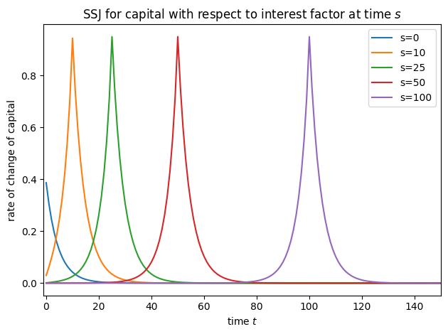
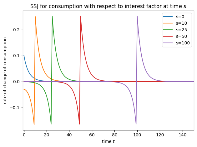
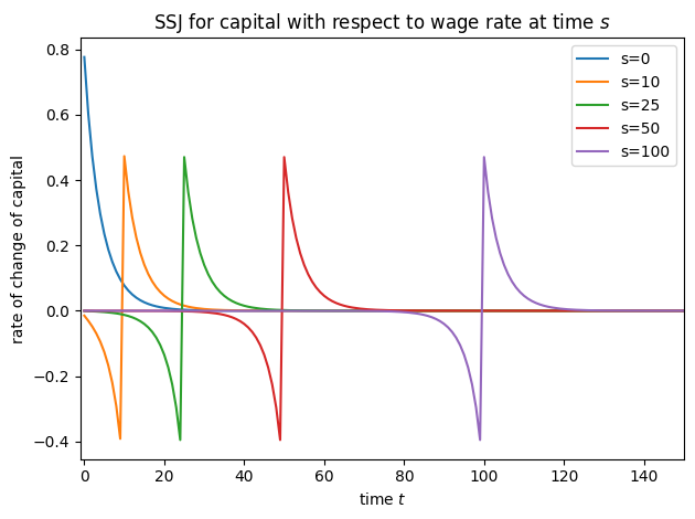
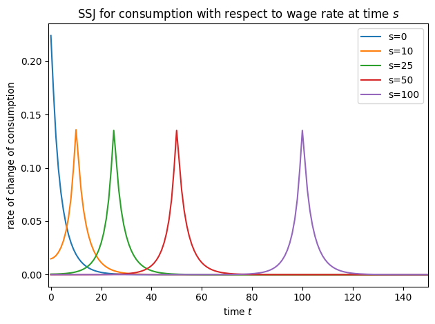
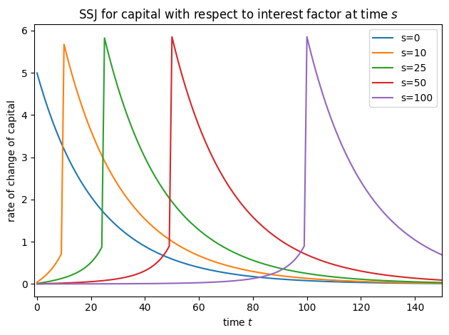
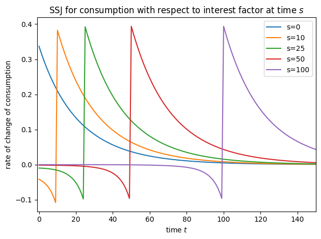
# Plot some slices of the SSJs
plot_SSJ(SSJ_K_r, [0, 10, 25, 50, 100], "capital", "interest factor", t_max=150)
plot_SSJ(SSJ_C_r, [0, 10, 25, 50, 100], "consumption", "interest factor", t_max=150)
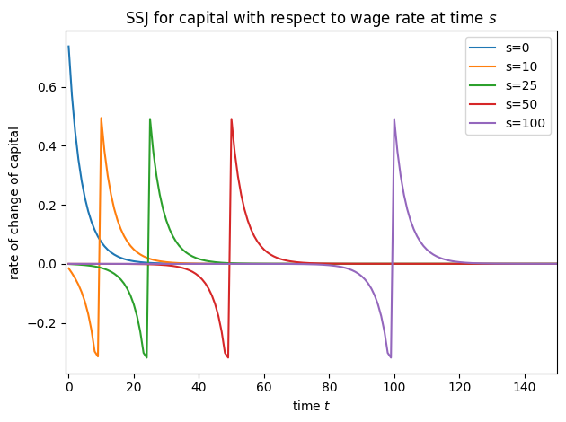
plot_SSJ(SSJ_K_w, [0, 10, 25, 50, 100], "capital", "wage rate", t_max=150)
plot_SSJ(SSJ_C_w, [0, 10, 25, 50, 100], "consumption", "wage rate", t_max=150)
In fact, the NewKeynesianConsumerType is simply a variation of IndShockConsumerType with this income process substituted in, and handwritten methods for computing SSJs for only assets and consumption. HARK’s new SSJ constructor method should work for (almost) all AgentType subclasses, and for any simulation output.
Adding Labor Supply on the Intensive Margin#
Now suppose you want to work with a properly new Keynesian macroeconomic environment, so that agents can vary the intensity of their labor supply depending on the wage rate (and their personal circumstances). The LaborIntMargConsumerType does just that, so let’s work with it.
[5]:
# Import and create an agent who chooses labor on the intensive margin
from HARK.ConsumptionSaving.ConsLaborModel import LaborIntMargConsumerType

LaborSupplyType = LaborIntMargConsumerType(cycles=0)
# This will raise some harmless warnings

# Make grid specifications
assets_grid_spec = {"min": 0.0, "max": 40.0, "N": 401}
labor_grid_spec = {"min": 0.0, "max": 2.0, "N": 201}
my_labor_grid_specs = {"kNrm": assets_grid_spec, "LbrEff": labor_grid_spec}
C:\Users\Matthew\Documents\GitHub\HARK\HARK\ConsumptionSaving\ConsLaborModel.py:146: RuntimeWarning: divide by zero encountered in divide
  * (bNrmGridTerm / (WageRte_T * TranShkGridTerm) + 1.0),
C:\Users\Matthew\Documents\GitHub\HARK\HARK\ConsumptionSaving\ConsLaborModel.py:146: RuntimeWarning: invalid value encountered in divide
  * (bNrmGridTerm / (WageRte_T * TranShkGridTerm) + 1.0),
C:\Users\Matthew\Documents\GitHub\HARK\HARK\rewards.py:66: RuntimeWarning: divide by zero encountered in power
  return c**-rho
[6]:
# Construct SSJs for capital and labor with respect to the interest factor and the wage rate
t0 = time()
SSJ_K_r, SSJ_L_r = LaborSupplyType.make_basic_SSJ(
    "Rfree",
    ["aNrm", "LbrEff"],
    my_labor_grid_specs,
    norm="PermShk",
    offset=True,
)
t1 = time()
print(
    "Constructing the SSJs with respect to the interest factor took {:.3f}".format(
        t1 - t0
    )
    + " seconds."
)

t0 = time()
SSJ_K_w, SSJ_L_w = LaborSupplyType.make_basic_SSJ(
    "WageRte",
    ["aNrm", "LbrEff"],
    my_labor_grid_specs,
    norm="PermShk",
    offset=True,
    solved=True,
)
t1 = time()
print(
    "Constructing the SSJs with respect to the wage rate took {:.3f}".format(t1 - t0)
    + " seconds."
)
Constructing the SSJs with respect to the interest factor took 42.820 seconds.
Constructing the SSJs with respect to the wage rate took 41.585 seconds.
Notice that the second time make_basic_SSJ is called, the argument solved=True is also passed. This is because the long run model is the same no matter what, so once it has been solved once (in the first call), we don’t need to re-solve it.
This model is a little less standard than the IndShockConsumerType, so let’s plot the policy functions so we’re familiar with what’s going on. Conveniently, LaborIntMargConsumerType has a couple of methods for quickly plotting its policy functions. The state variables at decision-time are bank balances \(b_t\) and the transitory productivity shock \(\theta_t\). The figures below plot the consumption function by \(b_t\) at various levels of transitory productivity.
[7]:
LaborSupplyType.plot_cFunc(0, bMax=10.0)
LaborSupplyType.plot_LbrFunc(0, bMax=10.0)
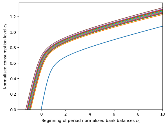
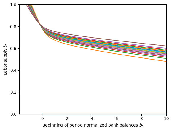
The blue curve that sits below all the others is for \(\theta_t=0\), representing unemployment at zero productivity; note the barely visible “zero labor supplied” curve in the second figure. The first figure might lead you to believe that this agent can borrow against future earnings, because their consumption function is defined for some \(b_t < 0\) when \(\theta_t > 0\), but this isn’t really the case. Note that for every level of \(\theta\), the consumption function goes to zero at exactly the same \(b_t\) as where the labor function goes to 1 (zero leisure). That minimum \(b_t\) represents the beginning-of-period wealth they need to have so that if they work 100% of the time and consume nothing, they will end the period with \(a_t=0\). Why is that important? Because productivity shocks are iid, and they might get \(\theta_{t+1}=0\); knowing that they need to be in a legal state in \(t+1\), the agent will never end their period with less than \(a_t = 0\) and risk having no resources next period while unemployed.
Also note that at levels of \(b_t\) that the agent will actually visit, labor supply is increasing in transitory productivity \(\theta_t\): the agent will work more when it’s a “good time to work”. Labor supply is also decreasing in \(b_t\). When the agent has more cash on hand already, they want to consume more and don’t need to work as much to finance that consumption. Note that a consequence of this is that a large permanent productivity shock \(\psi_t > 1\) will decrease normalized bank balances \(b_t\) and thus induce the agent to supply more labor– again, they will work more when it’s a “good time to work”.
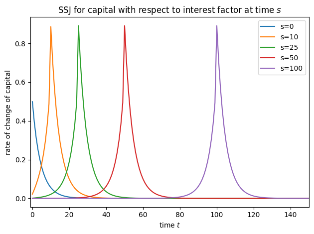
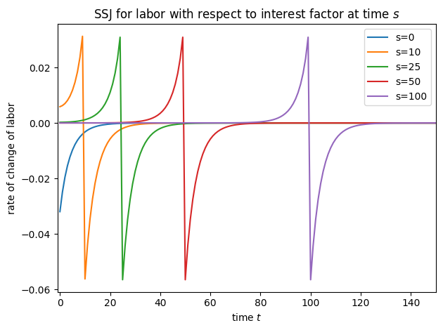
We provide all of that as prelude to plotting the SSJs, to aid in your interpretation of aggregate responses.
[8]:
# Plot some slices of the SSJs
plot_SSJ(SSJ_K_r, [0, 10, 25, 50, 100], "capital", "interest factor", t_max=150)
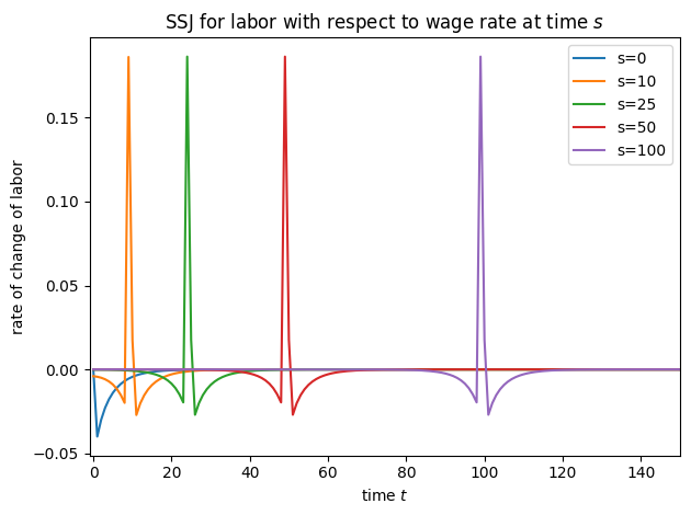
plot_SSJ(SSJ_L_r, [0, 10, 25, 50, 100], "labor", "interest factor", t_max=150)
plot_SSJ(SSJ_K_w, [0, 10, 25, 50, 100], "capital", "wage rate", t_max=150)
plot_SSJ(SSJ_L_w, [0, 10, 25, 50, 100], "labor", "wage rate", t_max=150)
Implementing Unemployment Dynamics#
Now suppose you’re interested in a model in which agents can be persistently unemployed, transitioning between employment and unemployment with known probabilities. In your macroeconomic environment, these transition probabilities might be determined endogenously, but from the perspective of one individual agent, they treat them as given.
HARK can handle this kind of model using its MarkovConsumerType, which adds a discrete state on top of the IndShockConsumerType model. Several model objects can depend on the discrete state: survival probabilities, the income shock distribution, the interest factor, and expected permanent income growth. Let’s make an instance of MarkovConsumerType with two discrete states, one for unemployment (zero labor income) and the other for employment, that are otherwise identical.
Conveniently, the default constructor for MrkvArray (the transition probabilities) is make_simple_binary_markov, so we don’t have to change much.
Let’s say that discrete state z=0 means unemployment and state z=1 means employment. The default IncShkDstn constructor for MarkovConsumerType is called construct_markov_lognormal_income_process_unemployment; it expects to get inputs for PermShkStd, TranShkStd, UnempPrb, and IncUnemp as they vary by discrete state z. We also need to make sure the discrete states don’t vary in any other way, and to set the persistence of (un)employment in the long run.
Because we might be interested in how interest rates affect aggregate outcomes, Rfree will be a shock parameter. Note that only real-valued parameters (or those in a singleton list) are eligible to be a shock, but Rfree is a list of arrays of interest factors by discrete state. There’s an easy fix for this: add a trivial constructor function for Rfree
[9]:
# Import our agent type
import numpy as np
from HARK.ConsumptionSaving.ConsMarkovModel import MarkovConsumerType
from HARK.distributions import DiscreteDistributionLabeled

# Specify parameters that differ from defaults
my_markov_params = {
    "PermShkStd": np.array([[0.1, 0.1]]),
    "TranShkStd": np.array([[0.1, 0.1]]),
    "UnempPrb": np.array([0.9999, 0.0]),
    "IncUnemp": np.array([0.0, 0.0]),
    "Mrkv_p11": [0.75],  # expect to be unemployed for 4 periods
    "Mrkv_p22": [0.985],  # expect to be employed for 67 periods
    "MrkvPrbsInit": np.array([0.1, 0.9]),
    "PermGroFac": [np.array([1.01, 1.01])],
    "LivPrb": [np.array([1.0, 1.0])],
    "Rfree_all": [1.03],  # a new parameter that we'll use to make Rfree!
    "DiscFac": 0.96,
    "tolerance": 1e-12,
}

# Define a substitute "unemployed" income distribution because the default constructor doesn't like zero income
UnemployedIncDstn = DiscreteDistributionLabeled(
    pmv=np.array([1.0]),
    atoms=np.array([[1.0], [0.0]]),
    var_names=["PermShk", "TranShk"],
)
[10]:
# Define a trivial constructor function for Rfree
def make_flat_Rfree(T_cycle, MrkvArray, Rfree_all):
    K = MrkvArray[0].shape[0]
    Rfree = T_cycle * [Rfree_all * np.ones(K)]
    return Rfree
[11]:
# Make and solve an infinite horizon problem with persistent unemployment
UnempDynType = MarkovConsumerType(cycles=0, **my_markov_params)
UnempDynType.IncShkDstn[0][0] = UnemployedIncDstn
UnempDynType.constructors["Rfree"] = make_flat_Rfree
UnempDynType.update()
UnempDynType.solve()
[12]:
# Plot the state-dependent consumption functions
UnempDynType.unpack("cFunc")
plt.xlabel(r"Normalized market resources $m_t$")
plt.ylabel(r"Normalized consumption $c_t$")
plt.ylim(0.0, 1.5)
plot_funcs(UnempDynType.cFunc[0], 0.0, 10.0)
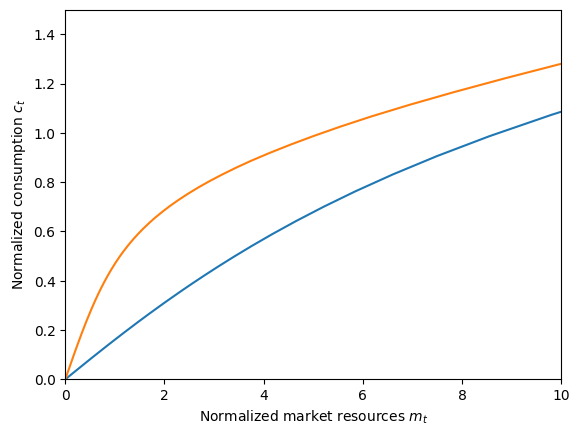
The orange plot is the consumption function when employed, and the blue plot is the consumption function when unemployed. For those familiar with Chris Carroll’s “tractable buffer stock” model, you might notice that the unemployed consumption function here looks a bit like the “unemployed” consumption function for the TBS model. This is sensible: being persistently unemployed with only a 25% chance of recovery each period is qualitatively related to knowing that you will never, ever receive labor income again.
Before proceeding to constructing the SSJs, let’s take a look at what the long run distribution of (arrival) states is for this model. The distribution we’re about to plot is actually constructed in the background as part of the process of making SSJs via the “fake news” algorithm, but hidden from the user. Let’s take a quick look at what’s happening “under the hood”.
[13]:
# Make grid specifications
assets_grid_spec = {"min": 0.0, "max": 60.0, "N": 401}
consumption_grid_spec = {"min": 0.0, "max": 3.0, "N": 301}
z_grid = {"N": 2}
my_mrkv_grid_specs = {
    "kNrm": assets_grid_spec,
    "cNrm": consumption_grid_spec,
    "zPrev": z_grid,
}
[14]:
# Find the steady state distribution and unpack it
UnempDynType.initialize_sym()
UnempDynType._simulator.make_transition_matrices(my_mrkv_grid_specs, norm="PermShk")
UnempDynType._simulator.find_steady_state()
kNrm_grid = UnempDynType._simulator.periods[0].grids["kNrm"]
SS_dstn = np.reshape(UnempDynType._simulator.steady_state_dstn, (401, 2))

# Plot the steady state distribution of capital
plt.plot(kNrm_grid, SS_dstn[:, 0], "-r", label="unemployed")
plt.plot(kNrm_grid, SS_dstn[:, 1], "-g", label="employed")
plt.xlabel(r"Beginning of period capital $k_t$")
plt.ylabel("Probability density")
plt.title("Long run distribution of capital holdings")
plt.legend()
plt.ylim(0.0, None)
plt.xlim(0.0, 25.0)
plt.show()
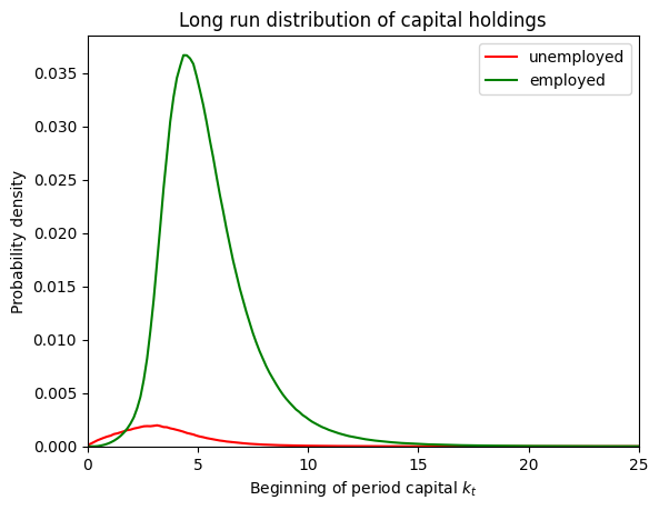
The SSJ constructor builds a representation of the model for simulation purposes (holding it in the _simulator attribute of the AgentType instance) and makes discretized transition matrices. The steady_state_dstn has size 802, or 401 capital gridpoints times 2 discrete states; the distribution is stored as a 1D vector but can be reshaped back into its “natural” form.
The grids that are built can also be used to calculate long run distributions of other outcomes. Let’s do a quick calculation of the steady state (un)employment rate in our specification.
[15]:
# Find the distributional mapping from arrival states to the discrete employment state
z_outcomes = UnempDynType._simulator.periods[0].matrices["z"]

# Combine the steady state distribution with that mapping
emp_dstn_LR = np.dot(SS_dstn.flatten(), z_outcomes)
print("The long run unemployed rate is {:.1f}".format(100 * emp_dstn_LR[0]) + "%.")
print("The long run employed rate is {:.1f}".format(100 * emp_dstn_LR[1]) + "%.")
The long run unemployed rate is 5.7%.
The long run employed rate is 94.3%.
If you do a hand calculation of the steady state (un)employment rate based on the dynamics we chose, you’ll get the same result!
Now we can make SSJs with respect to the interest factor and the persistence of (un)employment. Notice that the shock parameter for the interest rate is Rfree_all, the new parameter we defined above for use in the simple constructor function. When Rfree_all is perturbed, the change is applied through make_flat_Rfree to both discrete states. Likewise, we name the SSJ for (un)employment persistence UU or EE to be a bit more descriptive about what Mrkv_p11 and
Mrkv_p22 mean in this context.
[16]:
# Calculate SSJs with respect to the interest factor and (un)employment flows
t0 = time()
SSJ_K_r, SSJ_C_r = UnempDynType.make_basic_SSJ(
    "Rfree_all",
    ["aNrm", "cNrm"],
    my_mrkv_grid_specs,
    norm="PermShk",
    offset=True,
    solved=True,
)
t1 = time()
print(
    "Constructing the SSJs with respect to the interest factor took {:.3f}".format(
        t1 - t0
    )
    + " seconds."
)

t0 = time()
SSJ_K_UU, SSJ_C_UU = UnempDynType.make_basic_SSJ(
    "Mrkv_p11",
    ["aNrm", "cNrm"],
    my_mrkv_grid_specs,
    norm="PermShk",
    offset=True,
    solved=True,
)
t1 = time()
print(
    "Constructing the SSJs with respect to unemployment persistence took {:.3f}".format(
        t1 - t0
    )
    + " seconds."
)

t0 = time()
SSJ_K_EE, SSJ_C_EE = UnempDynType.make_basic_SSJ(
    "Mrkv_p22",
    ["aNrm", "cNrm"],
    my_mrkv_grid_specs,
    norm="PermShk",
    offset=True,
    solved=True,
)
t1 = time()
print(
    "Constructing the SSJs with respect to employment persistence took {:.3f}".format(
        t1 - t0
    )
    + " seconds in total."
)
Constructing the SSJs with respect to the interest factor took 36.190 seconds.
Constructing the SSJs with respect to unemployment persistence took 36.162 seconds.
Constructing the SSJs with respect to employment persistence took 35.882 seconds in total.
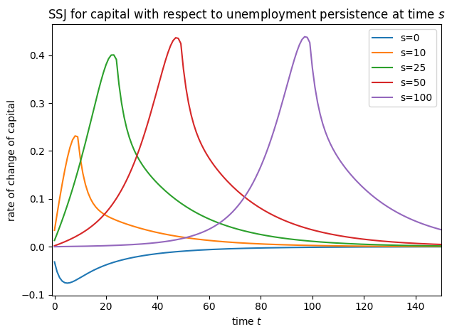
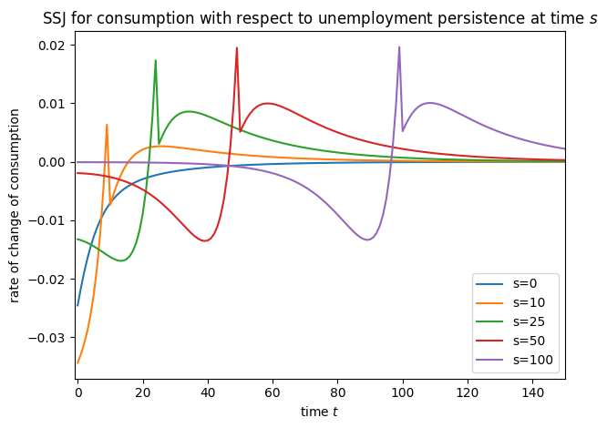
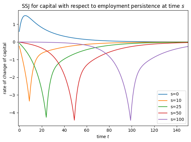
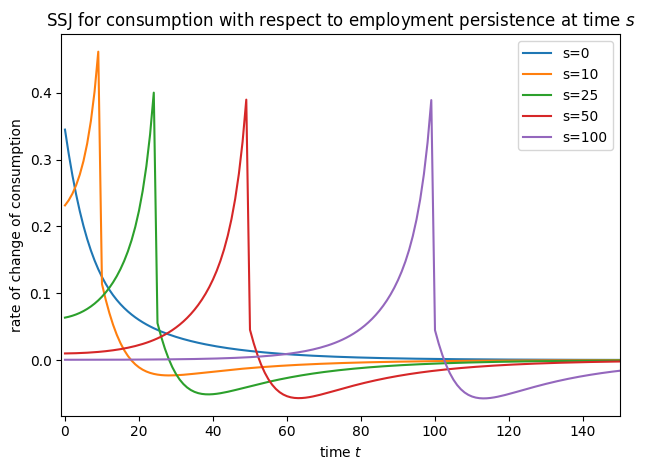
[17]:
# Plot some slices of the SSJs
plot_SSJ(
    SSJ_K_UU, [0, 10, 25, 50, 100], "capital", "unemployment persistence", t_max=150
)
plot_SSJ(
    SSJ_C_UU, [0, 10, 25, 50, 100], "consumption", "unemployment persistence", t_max=150
)
plot_SSJ(SSJ_K_EE, [0, 10, 25, 50, 100], "capital", "employment persistence", t_max=150)
plot_SSJ(
    SSJ_C_EE, [0, 10, 25, 50, 100], "consumption", "employment persistence", t_max=150
)
plot_SSJ(SSJ_K_r, [0, 10, 25, 50, 100], "capital", "interest factor", t_max=150)
plot_SSJ(SSJ_C_r, [0, 10, 25, 50, 100], "consumption", "interest factor", t_max=150)
SSJs with Portfolio Choice#
That was a lot of examples involving labor and employment, so let’s pivot to something on the capital side and consider a model with portfolio choice. Maybe you might be interested in a model in which agents can store their wealth in a low (or no) interest bond, or invest in risky assets– and only the risky asset is used to finance capital. HARK has a few models with portfolio allocation, but let’s use the simplest one, RiskyAssetConsumerType. Start by importing the AgentType subclass
and setting a few baseline parameters, then solve an infinite horizon problem.
[18]:
# Import our AgentType and then choose some parameters
from HARK.ConsumptionSaving.ConsRiskyAssetModel import RiskyAssetConsumerType

my_risky_params = {
    "RiskyShareFixed": None,
    "Rfree": [1.0],
    "RiskyAvg": 1.03,
    "RiskyStd": 0.26,
    "RiskyCount": 7,
    "LivPrb": [1.0],
    "CRRA": 3.5,
    "DiscFac": 0.97,
    "aXtraMax": 300.0,
    "aXtraCount": 200,
    "aXtraNestFac": 1,
    "tolerance": 1e-10,
}

# Make and solve our portfolio choice model
PortChoiceType = RiskyAssetConsumerType(cycles=0, **my_risky_params)
t0 = time()
PortChoiceType.solve()
t1 = time()
print(
    "Solving the portfolio allocation model took {:.3f}".format(t1 - t0) + " seconds."
)
Solving the portfolio allocation model took 40.581 seconds.
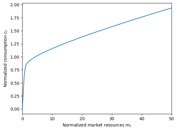
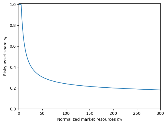
Let’s make sure the solution to the model looks sensible by plotting the policy functions.
[19]:
plt.xlabel(r"Normalized market resources $m_t$")
plt.ylabel(r"Normalized consumption $c_t$")
plot_funcs(PortChoiceType.solution[0].cFunc, 0.0, 50.0)

plt.ylim(0.0, 1.01)
plt.xlabel(r"Normalized market resources $m_t$")
plt.ylabel(r"Risky asset share $s_t$")
plot_funcs(PortChoiceType.solution[0].ShareFunc, 0.0, 300.0)
That looks ok to me. Now we can define grids for our outcomes of interest, then compute SSJs.
[20]:
assets_grid_spec = {"min": 0.0, "max": 100.0, "N": 501}
consumption_grid_spec = {"min": 0.0, "max": 3.0, "N": 201}
share_grid_spec = {"min": 0.0, "max": 1.0, "N": 101}
my_portfolio_grid_specs = {
    "kNrm": assets_grid_spec,
    "cNrm": consumption_grid_spec,
    "Share": share_grid_spec,
    "qNrm": assets_grid_spec,
}

t0 = time()
SSJ_K_r, SSJ_Q_r, SSJ_C_r = PortChoiceType.make_basic_SSJ(
    "RiskyAvg",
    ["aNrm", "qNrm", "cNrm"],
    my_portfolio_grid_specs,
    norm="PermShk",
    T_max=300,
    solved=True,
)
t1 = time()
print(
    "Constructing the SSJs with respect to mean risky return took {:.3f}".format(
        t1 - t0
    )
    + " seconds."
)

t0 = time()
SSJ_K_s, SSJ_Q_s, SSJ_C_s = PortChoiceType.make_basic_SSJ(
    "RiskyStd",
    ["aNrm", "qNrm", "cNrm"],
    my_portfolio_grid_specs,
    norm="PermShk",
    T_max=300,
    solved=True,
)
t1 = time()
print(
    "Constructing the SSJs with respect to stdev risky return took {:.3f}".format(
        t1 - t0
    )
    + " seconds."
)

t0 = time()
SSJ_K_f, SSJ_Q_f, SSJ_C_f = PortChoiceType.make_basic_SSJ(
    "Rfree",
    ["aNrm", "qNrm", "cNrm"],
    my_portfolio_grid_specs,
    norm="PermShk",
    T_max=300,
    solved=True,
)
t1 = time()
print(
    "Constructing the SSJs with respect to risk-free return return took {:.3f}".format(
        t1 - t0
    )
    + " seconds."
)
Constructing the SSJs with respect to mean risky return took 88.749 seconds.
Constructing the SSJs with respect to stdev risky return took 89.499 seconds.
Constructing the SSJs with respect to risk-free return return took 87.929 seconds.
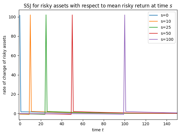
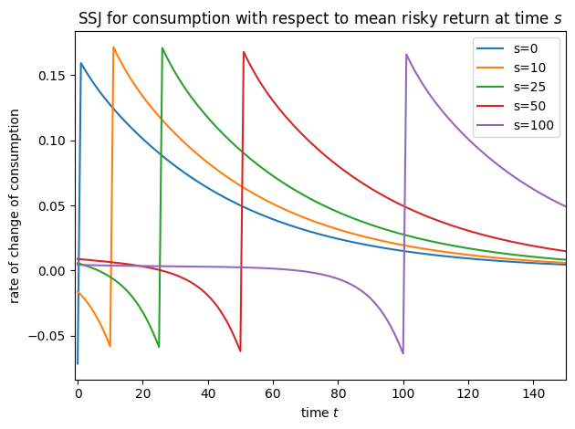
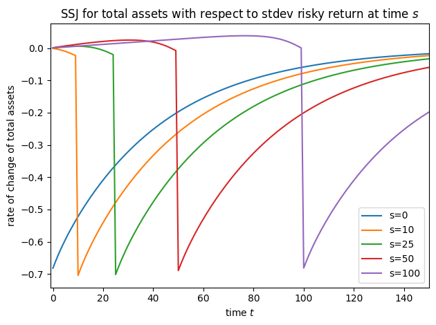
[21]:
# Plot some slices of the SSJs
plot_SSJ(SSJ_K_r, [0, 10, 25, 50, 100], "total assets", "mean risky return", t_max=150)
plot_SSJ(SSJ_Q_r, [0, 10, 25, 50, 100], "risky assets", "mean risky return", t_max=150)
plot_SSJ(SSJ_C_r, [0, 10, 25, 50, 100], "consumption", "mean risky return", t_max=150)
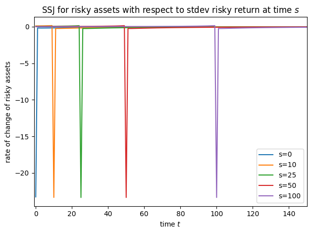
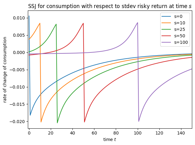
plot_SSJ(SSJ_K_s, [0, 10, 25, 50, 100], "total assets", "stdev risky return", t_max=150)
plot_SSJ(SSJ_Q_s, [0, 10, 25, 50, 100], "risky assets", "stdev risky return", t_max=150)
plot_SSJ(SSJ_C_s, [0, 10, 25, 50, 100], "consumption", "stdev risky return", t_max=150)
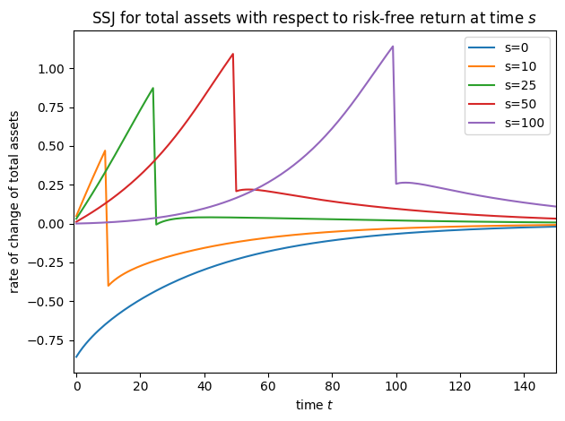
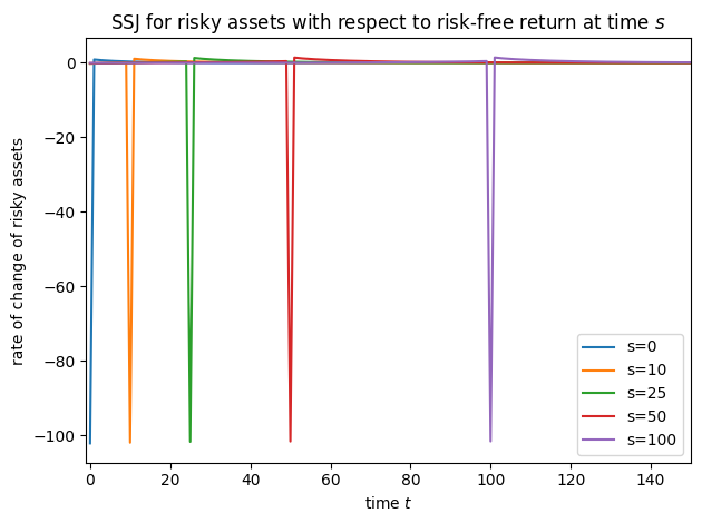
plot_SSJ(SSJ_K_f, [0, 10, 25, 50, 100], "total assets", "risk-free return", t_max=150)
plot_SSJ(SSJ_Q_f, [0, 10, 25, 50, 100], "risky assets", "risk-free return", t_max=150)
plot_SSJ(SSJ_C_f, [0, 10, 25, 50, 100], "consumption", "risk-free return", t_max=150)
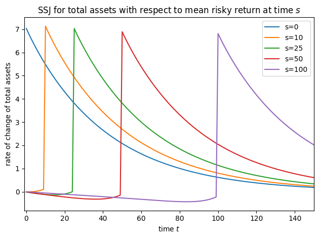
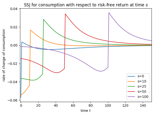
Note that for this model, we did not specify offset=True when constructing SSJs, but we did set it for interest factor shocks in all other models– why?! It’s because of a quirk of the timing of the model file. In the risky asset model, the model file says that the risky interest factor is revealed at the end of the period; in all other models, the interest factor is applied to capital at the start of the period. We change the timing for this model so that the risky asset share does
not need to be “carried over” as an arrival variable in \(t+1\), but instead used in the same \(t\) where it was chosen. This reduces the dimensionality of the model from the perspective of the intertemporal transition.
To see this difference in model timing, let’s use the describe_model() method on the risky asset consumer and a different agent type.
[22]:
PortChoiceType.describe_model()
ConsRiskyAsset: Consumption-saving model with permanent and transitory income risk and asset allocation between a risk-free asset and a (higher return) risky asset. In this simple model, asset returns happen at the *end* of a period. This will only work properly if income and return shocks are independent.

----------------------------------
%%%%%%%%%%%%% SYMBOLS %%%%%%%%%%%%
----------------------------------
kNrm (float)        : beginning of period wealth, normalized by p_{t-1}
pLvlPrev (float)    : inbound permanent income level, before growth
Risky (float)       : realized return factor on risky assets
Rport (float)       : realized return factor on portfolio
yNrm (float)        : normalized labor income
pLvl (float)        : permanent income level
bNrm (float)        : normalized bank balances
mNrm (float)        : normalized market resources
cNrm (float)        : normalized consumption
Share (float)       : share of wealth allocated to risky assets this period
aNrm (float)        : normalized end-of-period assets
qNrm (float)        : normalized risky asset holdings
live (bool)         : whether the agent survives
Rfree (param)       : risk free return factor on assets
PermGroFac (param)  : expected permanent income growth factor
LivPrb (param)      : survival probability at end of period
cFunc (func)        : consumption function over market resources
ShareFunc (func)    : risky share function over market resource
IncShkDstn (dstn)   : joint distribution of permanent and transitory income shocks
RiskyDstn (dstn)    : distribution of risky asset returns
pLvlInitDstn (dstn) : distribution of permanent income at model birth
kNrmInitDstn (dstn) : distribution of normalized capital holdings at birth
PermShk (float)     :
TranShk (float)     :
G (float)           :
wNrm (float)        :
dead (bool)         : whether agent died this period
t_seq (int)         : which period of the sequence the agent is on
t_age (int)         : how many periods the agent has already lived for
----------------------------------
%%%%% INITIALIZATION AT BIRTH %%%%
----------------------------------
pLvlPrev ~ pLvlInitDstn : draw initial permanent income from distribution
kNrm ~ kNrmInitDstn     : draw initial capital from distribution
----------------------------------
%%%% DYNAMICS WITHIN PERIOD t %%%%
----------------------------------
(PermShk,TranShk) ~ IncShkDstn    : draw income shocks from joint distribution
yNrm = TranShk                    : normalized income is the transitory shock
G = PermGroFac*PermShk            : calculate permanent income growth
pLvl = pLvlPrev*G                 : update permanent income level
bNrm = kNrm/G                     : calculate normalized bank balances
mNrm = bNrm+yNrm                  : calculate normalized market resources
cNrm = cFunc@(mNrm)               : evaluate consumption when share is fixed
Share = ShareFunc@(mNrm)          : evaluate risky share when it is fixed
wNrm = mNrm-cNrm                  : calculate wealth after consumption
Risky ~ RiskyDstn                 : draw risky return shock
Rport = Rfree+(Risky-Rfree)*Share : calculate realized portfolio return
aNrm = Rport*wNrm                 : calculate end-of-period assets
qNrm = aNrm*Share                 : calculate risky asset holdings
live ~ {LivPrb}                   : draw survival
dead = 1-live                     : dead are non-survivors
----------------------------------
%%%%%%% RELABELING / TWIST %%%%%%%
----------------------------------
aNrm[t-1] <---> kNrm[t]
pLvl[t-1] <---> pLvlPrev[t]
-----------------------------------
[23]:
IndShkTypeWithWage.describe_model()
ConsIndShock: Consumption-saving model with permanent and transitory income shocks and a risk-free asset.

----------------------------------
%%%%%%%%%%%%% SYMBOLS %%%%%%%%%%%%
----------------------------------
kNrm (float)        : beginning of period capital, normalized by p_{t-1}
pLvlPrev (float)    : inbound permanent income level, before growth
yNrm (float)        : normalized labor income
pLvl (float)        : permanent income level
bNrm (float)        : normalized bank balances
mNrm (float)        : normalized market resources
cNrm (float)        : normalized consumption
aNrm (float)        : normalized end-of-period assets
live (bool)         : whether the agent survives
Rfree (param)       : risk free return factor on assets
PermGroFac (param)  : expected permanent income growth factor
LivPrb (param)      : survival probability at end of period
cFunc (func)        : consumption function over market resources
IncShkDstn (dstn)   : joint distribution of permanent and transitory shocks
pLvlInitDstn (dstn) : distribution of permanent income at model birth
kNrmInitDstn (dstn) : distribution of normalized capital holdings at birth
PermShk (float)     :
TranShk (float)     :
G (float)           :
dead (bool)         : whether agent died this period
t_seq (int)         : which period of the sequence the agent is on
t_age (int)         : how many periods the agent has already lived for
----------------------------------
%%%%% INITIALIZATION AT BIRTH %%%%
----------------------------------
pLvlPrev ~ pLvlInitDstn : draw initial permanent income from distribution
kNrm ~ kNrmInitDstn     : draw initial capital from distribution
----------------------------------
%%%% DYNAMICS WITHIN PERIOD t %%%%
----------------------------------
(PermShk,TranShk) ~ IncShkDstn : draw permanent and transitory income shocks
yNrm = TranShk                 : normalized income is the transitory shock
G = PermGroFac*PermShk         : calculate permanent income growth
pLvl = pLvlPrev*G              : update permanent income level
bNrm = Rfree*kNrm/G            : calculate normalized bank balances
mNrm = bNrm+yNrm               : calculate normalized market resources
cNrm = cFunc@(mNrm)            : evaluate consumption from market resources
aNrm = mNrm-cNrm               : calculate normalized end-of-period assets
live ~ {LivPrb}                : draw survival
dead = 1-live                  : dead are non-survivors
----------------------------------
%%%%%%% RELABELING / TWIST %%%%%%%
----------------------------------
aNrm[t-1] <---> kNrm[t]
pLvl[t-1] <---> pLvlPrev[t]
-----------------------------------