Interactive online version:
Making HA-SSJ Matrices with HARK#
Background on HA-SSJs#
HARK has functionality for constructing heterogeneous agent sequence space Jacobian (HA-SSJ) matrices for its various AgentType subclasses. If you don’t know what an SSJ is, see “Using the Sequence-Space Jacobian to Solve and Estimate Heterogeneous-Agent Models” by Auclert, Bardoczy, Rognlie, and Straub (Ecma 2021); see also our overview notebook here.
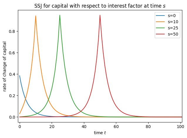
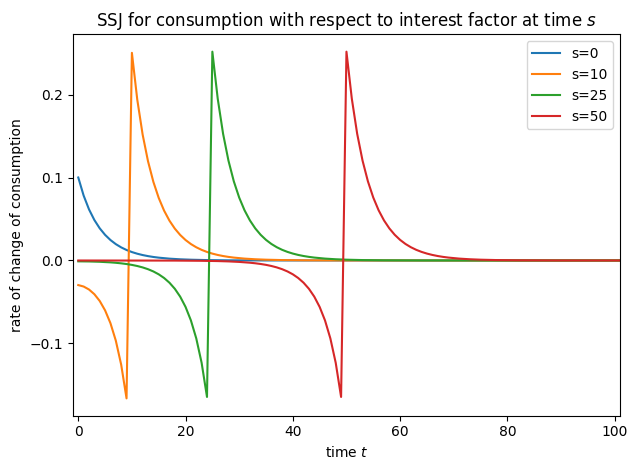
The very short version is that an HA-SSJ is the matrix of first derivatives of some HA model output with respect to some model input across periods. Suppose we are interested in some scalar \(Y_t\)– some outcome of the agents’ model– and how it changes with some model input \(x_s\) that can vary across time (both \(t\) and \(s\) are time subscripts). For example, \(Y\) might be average capital holdings, and \(x\) might be the interest factor. The HA-SSJ of \(Y\) with respect to \(x\) is a \(T \times T\) matrix denoted \(\mathcal{J}^{Y,x}\) for some time horizon \(T\). Element \(t,s\) of the Jacobian represents the rate at which \(Y_t\) changes with a change in \(x_s\) if the agents learn this information at \(t=0\) when in some long run steady state.
Collectively, all relevant HA-SSJs for a given model represent the dynamic behavior of aggregated microeconomic outcomes with respect to aggregate inputs to first order. In their paper, Auclert et al show that when combined with analogous objects at the economy level, HA-SSJs can be used to quickly compute model impulse responses with incredible accuracy. They also provide an efficient algorithm for calculating HA-SSJs for a wide class of microeconomic models. Econ-ARK has implemented their
“fake news” algorithm in HARK, so that HA-SSJs can be automatically computed for any and all AgentType subclasses (for which this is appropriate) with minimal user effort.
Very recently, Bence Bardoczy and Mateo Velasquez-Giraldo have extended the methodology to life-cycle frameworks, whereas the original Auclert et al paper addressed only standard infinite horizon models. The construction of HA-SSJs for life-cycle models has now been incorporated into HARK as well.
A First Example#
More details will be provided below, but let’s start with a very simple example. We’ll use IndShockConsumerType, the canonical consumption-saving problem with a permanent-transitory income shocks structure (sometimes referred to as the “Friedman buffer stock” income process) and one risk free asset with return factor Rfree.
In the code cells below, the SSJs for aggregate asset holdings (capital) and aggregate consumption are constructed with respect to the interest factor using the make_basic_SSJ() method, for a standard infinite horizon model. If you are interested in using HA-SSJs in the context of a life-cycle model, please see our notebook about that.
[1]:
# Import our AgentType subclass and basic tools
from HARK.ConsumptionSaving.ConsIndShockModel import IndShockConsumerType
from HARK.utilities import plot_SSJ
from time import time
import matplotlib.pyplot as plt
[2]:
# Initialize an infinite horizon AgentType instance
MyType = IndShockConsumerType(cycles=0, tolerance=1e-12)

# Make a dictionary of grid specifications
assets_grid_spec = {"min": 0.0, "max": 40.0, "N": 301, "order": 2.5}
consumption_grid_spec = {"min": 0.0, "max": 3.0, "N": 201}
my_grid_specs = {"kNrm": assets_grid_spec, "cNrm": consumption_grid_spec}
[3]:
# Compute the SSJs and time it
t0 = time()
SSJ_K_r, SSJ_C_r = MyType.make_basic_SSJ(
    "Rfree",  # name of the parameter to be shocked
    ["aNrm", "cNrm"],  # name(s) of the outcome variable(s) we're interested in
    my_grid_specs,  # dictionary of grid specifications
    norm="PermShk",
    offset=True,
)
t1 = time()

print("Constructing those SSJs took {:.3f}".format(t1 - t0) + " seconds in total.")
Constructing those SSJs took 11.669 seconds in total.
[4]:
# Plot select columns of the HA-SSJs
plot_SSJ(SSJ_K_r, [0, 10, 25, 50], "capital", "interest factor", t_max=100)
plot_SSJ(SSJ_C_r, [0, 10, 25, 50], "consumption", "interest factor", t_max=100)
Basic SSJ Functionality#
The AgentType class (and thus its many subclasses) has a make_basic_SSJ() method. It is “basic” in the sense that it only works for “standard” infinite horizon models (as in the original Auclert et al paper), and for life-cycle models with “flat” population dynamics (as in the Bardoczy and Velasquez-Giraldo paper).
A “standard” infinite horizon model is one that has the same kind of period happens over and over again, as in a typical infinite horizon or perpetual youth model, rather than a sequence of several different periods happening in a loop (e.g., seasonal effects). In HARK terms, the AgentType instance must have cycles=0 (infinite horizon) and T_cycle=1 (one period repeated indefinitely), or the method will terminate with an error immediately.
By “flat” population dynamics in a life-cycle model (cycles=1), we mean that survival in the model is not endogenous to agent behavior (e.g., via endogenous health), and that any shocks that you are interested in do not affect survival directly or indirectly. Essentially, the population mass that survives to each age must be independent of the shocks. In the future, the restriction to “flat” population dynamics will be generalized.
Suppose you have an AgentType instance called ThisType. When you call ThisType.make_basic_SSJ(), you must pass the following three arguments:
shock: The name of the variable that the SSJ(s) will be computed with respect to; this is \(x\) from above. This doesn’t have to be a “shock” in the modeling sense of “a random variable that will realize at some point”, but it does have to be a parameter that affects the agent’s problem. See below for more.outcomes: The name (or a list of names) of outcome variables for which SSJs will be constructed; this is \(Y\) from above. These must be variables that are realized during model simulation, and the outcome of interest is their population average.grids: A dictionary of grid specifications to be used. The keys of this dictionary are the names of model variables, including both arrival variables and outcomes of interest. The entries are dictionaries with grid information for that variable. If the variable is real-valued, then the dictionary should include amin,max, andN, and the grid will be equispaced by default. Optionally, specifying a re-valuedorder\(> 0\) makes a polynomially spaced grid (higher orders have gridpoints more tightly clustered near the bottom); alternatively, specifying a positive integer fornestdesignates the grid as multi-exponentially spaced (with that many layers of nesting). If the variable is discrete, then the dictionary needs only anNentry, and the values are assumed to be \(0,..,N-1\). The user must provide grid specifications for all arrival variables (except one that is normalized with the “Harmenberg trick”, see below), as well as for anyoutcomesthat are not continuation variables. If a namedoutcomeis a continuation variable, (e.g.aNrm), then its grid specification is the same as the corresponding arrival variable (e.g.kNrm).
You can also pass the following optional arguments, which have defaults in parentheses:
eps(0.0001) : The SSJ constructor uses one-sided first differences for computing derivatives. Theepsinput selects the amount by which to perturbshockwhen doing so.T_max(300) : The time horizon of the SSJs, and thus the size of the square matrices that are generated. The method assumes that the model returns to the long run steady state at \(t=T\) and beyond. See Auclert et al for a discussion of how to select the time horizon.norm(None) : The name of the model variable to normalize by for “Harmenberg aggregation”, if any. For many HARK models, this should be'PermShk', which enables the grid over permanent income to be omitted as an explicit state. See discussion below for caveats.solved(False) : Whether the agent’s long run problem has already been solved (by calling itssolve()method). Setting this to True is useful to save a little bit of time when computing SSJs for several shocks, as the long run model is the same for all of them.offset(False) : Whether the model input that is perturbed is “offset in time” and is actually indexed by \(t+1\) from HARK’s perspective. This usually includes anything that pertains to dynamics that happen at the start of a period, before the choice is made.construct(True) : Whether the agent’sconstructorupdatemethod should be called after theshockis updated. To be safe, this should be left at its default. A (very) small amount of time can be saved if theshockvariable is a direct model input and not used to construct any other model inputs.verbose(False) : Whether to print information about the method’s progress and timing to screen. When working with a new model, we recommend that you set this toTrueso that you can see a bit more about what’s happening.
How Do I Know What the Model Variables Are Called?#
To make an SSJ, the user needs to specify what outcomes they’re interested in and what variable is being perturbed (the “shock”); how are they supposed to know what these variables are called? Under the hood, the SSJ constructor uses a description of the model specified in a model file in HARK. To view information about the content of the model file, including descriptions of the various variables that are realized during simulation, just call the describe_model() method on your
AgentType instance. Any variable (but not distributions or functions) named in the SYMBOLS section can have a grid specified for it and be an outcome variable.
We said above that all real-valued arrival variables must have a grid specified. What’s an “arrival variable”? It’s an idiosyncratic variable that’s inbound into a period, existing at the very start of time \(t\). For “newborn” agents who were just created, these values are initialized as specified in the INITIALIZATION AT BIRTH section. For other agents, arrival variables are “carried over” from the prior period’s continuation variables. In the model description, you should see
all arrival variables set to some value (or drawn from a distribution) in the INITIALIZATION section. At the bottom, the RELABELING / TWIST section shows the relationships between continuation variables at \(t-1\) and arrival variables in \(t\) (for non-newborns).
[5]:
# Get a description of the model
MyType.describe_model()
ConsIndShock: Consumption-saving model with permanent and transitory income shocks and a risk-free asset.

----------------------------------
%%%%%%%%%%%%% SYMBOLS %%%%%%%%%%%%
----------------------------------
kNrm (float)        : beginning of period capital, normalized by p_{t-1}
pLvlPrev (float)    : inbound permanent income level, before growth
yNrm (float)        : normalized labor income
pLvl (float)        : permanent income level
bNrm (float)        : normalized bank balances
mNrm (float)        : normalized market resources
cNrm (float)        : normalized consumption
aNrm (float)        : normalized end-of-period assets
live (bool)         : whether the agent survives
Rfree (param)       : risk free return factor on assets
PermGroFac (param)  : expected permanent income growth factor
LivPrb (param)      : survival probability at end of period
cFunc (func)        : consumption function over market resources
IncShkDstn (dstn)   : joint distribution of permanent and transitory shocks
pLvlInitDstn (dstn) : distribution of permanent income at model birth
kNrmInitDstn (dstn) : distribution of normalized capital holdings at birth
PermShk (float)     :
TranShk (float)     :
G (float)           :
dead (bool)         : whether agent died this period
t_seq (int)         : which period of the sequence the agent is on
t_age (int)         : how many periods the agent has already lived for
----------------------------------
%%%%% INITIALIZATION AT BIRTH %%%%
----------------------------------
pLvlPrev ~ pLvlInitDstn : draw initial permanent income from distribution
kNrm ~ kNrmInitDstn     : draw initial capital from distribution
----------------------------------
%%%% DYNAMICS WITHIN PERIOD t %%%%
----------------------------------
(PermShk,TranShk) ~ IncShkDstn : draw permanent and transitory income shocks
yNrm = TranShk                 : normalized income is the transitory shock
G = PermGroFac*PermShk         : calculate permanent income growth
pLvl = pLvlPrev*G              : update permanent income level
bNrm = Rfree*kNrm/G            : calculate normalized bank balances
mNrm = bNrm+yNrm               : calculate normalized market resources
cNrm = cFunc@(mNrm)            : evaluate consumption from market resources
aNrm = mNrm-cNrm               : calculate normalized end-of-period assets
live ~ {LivPrb}                : draw survival
dead = 1-live                  : dead are non-survivors
----------------------------------
%%%%%%% RELABELING / TWIST %%%%%%%
----------------------------------
aNrm[t-1] <---> kNrm[t]
pLvl[t-1] <---> pLvlPrev[t]
-----------------------------------
What Can Be Used As a Shock Variable?#
Learning what can be used as a shock variable for an SSJ (the information that’s being perturbed) is a little more difficult. It’s tempting to look at the model description and assume that anything that’s listed as a param in the SYMBOLS section can be named as the shock, but that’s an oversimplification. You can choose as the shock any parameter that is real-valued, including those that live in a singleton list (say, because they’re time-varying). That includes some of the
parameters listed in the model description, but not necessarily all… and it also includes a bunch of other parameters that don’t appear in the description anywhere!
In HARK models, some parameters are “direct” in the sense that they are used literally as-is; the intertemporal discount factor DiscFac is (usually) simply specified as a real number, and that’s that. However, other parameters are “indirect” because they are used to construct other objects used by the model. For example, the default income shock process for IndShockConsumerType uses parameters called PermShkStd, TranShkStd, IncUnemp, UnempPrb, etc. None of those
parameters are named in the model description, but they are passed to a constructor function to build the contents of IncShkDstn at instantiation and whenever the construct() method is called. That constructor lives in the constructors dictionary attribute of each AgentType instance.
A quick way to find the names of the inputs for a constructor function is to use the get_arg_names convenience function. To interpret those argument names, you might try using Python’s built-in help function, which prints an object’s docstring (if any). Most constructors used by HARK by default should have descriptive docstrings.
[6]:
from HARK.core import get_arg_names

print(get_arg_names(MyType.constructors["IncShkDstn"]))
('T_cycle', 'PermShkStd', 'PermShkCount', 'TranShkStd', 'TranShkCount', 'T_retire', 'UnempPrb', 'IncUnemp', 'UnempPrbRet', 'IncUnempRet', 'RNG', 'neutral_measure')
[7]:
help(MyType.constructors["IncShkDstn"])
Help on function construct_lognormal_income_process_unemployment in module HARK.Calibration.Income.IncomeProcesses:

construct_lognormal_income_process_unemployment(T_cycle, PermShkStd, PermShkCount, TranShkStd, TranShkCount, T_retire, UnempPrb, IncUnemp, UnempPrbRet, IncUnempRet, RNG, neutral_measure=False)
    Generates a list of discrete approximations to the income process for each
    life period, from end of life to beginning of life.  Permanent shocks (:math:`\psi`) are mean
    one lognormally distributed with standard deviation PermShkStd[t] during the
    working life, and degenerate at 1 in the retirement period. Transitory shocks (:math:`\theta`)
    are mean one lognormally distributed with a point mass at IncUnemp with
    probability UnempPrb while working; they are mean one with a point mass at
    IncUnempRet with probability UnempPrbRet.  Retirement occurs
    after t=T_retire periods of working.

    .. math::
        \begin{align*}
        \psi_t &\sim \begin{cases}
        \exp(\mathcal{N}(-\textbf{PermShkStd}_{t}^{2}/2,\textbf{PermShkStd}_{t}^{2})) & \text{if } t \leq t_{\text{retire}}\\
        1 & \text{if } t > t_{\text{retire}}
        \end{cases}\\
        p_{\text{unemp}} & = \begin{cases}
        \textbf{UnempPrb} & \text{if } t \leq t_{\text{retire}} \\
        \textbf{UnempPrbRet} & \text{if } t > t_{\text{retire}} \\
        \end{cases}\\
        &\text{if } p > p_{\text{unemp}} \\
        \theta_t &\sim\begin{cases}
        \exp(\mathcal{N}(-\textbf{PermShkStd}_{t}^{2}/2-\ln(\frac{1-\textbf{IncUnemp }\textbf{UnempPrb}}{1-\textbf{UnempPrb}}),\textbf{PermShkStd}_{t}^{2})) & \text{if } t\leq t_{\text{retire}}\\
        \frac{1-\textbf{UnempPrbRet }\textbf{IncUnempRet}}{1-\textbf{UnempPrbRet}} & \text{if } t > t_{\text{retire}} \\
        \end{cases}\\
        &\text{otherwise}\\
        \theta_t &\sim\begin{cases}
        \textbf{IncUnemp} & \text{if } t\leq t_{\text{retire}}\\
        \textbf{IncUnempRet} & \text{if } t\leq t_{\text{retire}}\\
        \end{cases}\\
        \mathbb{E}[\psi]&=\mathbb{E}[\theta] = 1.\\
        \end{align*}

    All time in this function runs forward, from t=0 to t=T

    Parameters
    ----------
    PermShkStd : [float]
        List of standard deviations in log permanent income uncertainty during
        the agent's life.
    PermShkCount : int
        The number of approximation points to be used in the discrete approximation
        to the permanent income shock distribution.
    TranShkStd : [float]
        List of standard deviations in log transitory income uncertainty during
        the agent's life.
    TranShkCount : int
        The number of approximation points to be used in the discrete approximation
        to the permanent income shock distribution.
    UnempPrb : float or [float]
        The probability of becoming unemployed during the working period.
    UnempPrbRet : float or None
        The probability of not receiving typical retirement income when retired.
    T_retire : int
        The index value for the final working period in the agent's life.
        If T_retire <= 0 then there is no retirement.
    IncUnemp : float or [float]
        Transitory income received when unemployed.
    IncUnempRet : float or None
        Transitory income received while "unemployed" when retired.
    T_cycle :  int
        Total number of non-terminal periods in the consumer's sequence of periods.
    RNG : np.random.RandomState
        Random number generator for this type.
    neutral_measure : bool
        Indicator for whether the permanent-income-neutral measure should be used.

    Returns
    -------
    IncShkDstn :  [distribution.Distribution]
        A list with T_cycle elements, each of which is a
        discrete approximation to the income process in a period.
For more information about the constructors for your AgentType instance, you can invoke its describe_constructors() method, optionally passing one or more constructed object names (passing no arguments will display information about all constructors). A checkmark means that the constructed object (or its corresponding requirement) means that it exists; an X means that it has not been constructed and does not exist, and an asterisk means that the input does not exist, but the constructor
function has a specified default value for it.
[8]:
MyType.describe_constructors()
✓ kNrmInitDstn : make_lognormal_kNrm_init_dstn
    ✓ kLogInitMean
    ✓ kLogInitStd
    ✓ kNrmInitCount
    ✓ RNG
✓ pLvlInitDstn : make_lognormal_pLvl_init_dstn
    ✓ pLogInitMean
    ✓ pLogInitStd
    ✓ pLvlInitCount
    ✓ RNG
✓ IncShkDstn : construct_lognormal_income_process_unemployment
    ✓ T_cycle
    ✓ PermShkStd
    ✓ PermShkCount
    ✓ TranShkStd
    ✓ TranShkCount
    ✓ T_retire
    ✓ UnempPrb
    ✓ IncUnemp
    ✓ UnempPrbRet
    ✓ IncUnempRet
    ✓ RNG
    ✓ neutral_measure
✓ PermShkDstn : get_PermShkDstn_from_IncShkDstn
    ✓ IncShkDstn
    ✓ RNG
✓ TranShkDstn : get_TranShkDstn_from_IncShkDstn
    ✓ IncShkDstn
    ✓ RNG
✓ aXtraGrid : make_assets_grid
    ✓ aXtraMin
    ✓ aXtraMax
    ✓ aXtraCount
    ✓ aXtraExtra
    ✓ aXtraNestFac
✓ solution_terminal : make_basic_CRRA_solution_terminal
    ✓ CRRA
Any constructor inputs that are a single float or a singleton list of one float are eligible to be named as a shock variable. Note that in more complex models, some constructor arguments could be constructed by another constructor! In such cases, you might need to look at another constructor to find the “basic” or “primitive” parameter that you want to be your shock.
To see which model objects have constructors, simply do list(MyType.constructors.keys()). If you want to know the names of the functions (and where their source code can be found), look at MyType.constructors.
[9]:
print("Constructed objects are:", list(MyType.constructors.keys()))
for key in MyType.constructors.keys():
    print(key + " : " + str(MyType.constructors[key]))
Constructed objects are: ['kNrmInitDstn', 'pLvlInitDstn', 'IncShkDstn', 'PermShkDstn', 'TranShkDstn', 'aXtraGrid', 'solution_terminal']
kNrmInitDstn : <function make_lognormal_kNrm_init_dstn at 0x000001ADCE92A7A0>
pLvlInitDstn : <function make_lognormal_pLvl_init_dstn at 0x000001ADCE9E6AC0>
IncShkDstn : <function construct_lognormal_income_process_unemployment at 0x000001ADCE9E5800>
PermShkDstn : <function get_PermShkDstn_from_IncShkDstn at 0x000001ADCE9E5A80>
TranShkDstn : <function get_TranShkDstn_from_IncShkDstn at 0x000001ADCE9E5B20>
aXtraGrid : <function make_assets_grid at 0x000001ADCC32D800>
solution_terminal : <function make_basic_CRRA_solution_terminal at 0x000001ADCE9E7420>
One quick way to more or less get a list of all parameters that can be the shock is to look at your AgentType subclass’ default parameters, which are stored in the attribute default_["params"]. Essentially every entry there that is a float or singleton list with one float can be a shock parameter. Of course, not all of them are interesting or relevant as a shock– we can’t imagine what it means economically for the lower bound of the aNrm grid (when solving)
to change in the future!
Moreover, a very small number of parameters that are otherwise eligible to be named as the shock should not be used in this way, because HARK’s solution methods assume that these parameters are constant within a person. The primary example of this is CRRA, the coefficient of relative risk aversion. We don’t think of this as something that can be changed by economic events in the future, but nothing computationally prevents a user from asking for SSJs with respect to CRRA. However,
the output produced will be incorrect, and in some cases the finite horizon model solver might fail during the fake news algorithm.
[10]:
for key in list(MyType.default_["params"].keys()):
    if key == "constructors":
        continue  # skip this, it's shown above
    print(key + " : " + str(MyType.default_["params"][key]))
PermShkStd : [0.1]
PermShkCount : 7
TranShkStd : [0.1]
TranShkCount : 7
UnempPrb : 0.05
IncUnemp : 0.3
T_retire : 0
UnempPrbRet : 0.005
IncUnempRet : 0.0
kLogInitMean : -12.0
kLogInitStd : 0.0
kNrmInitCount : 15
pLogInitMean : 0.0
pLogInitStd : 0.0
pLvlInitCount : 15
aXtraMin : 0.001
aXtraMax : 20
aXtraNestFac : 3
aXtraCount : 48
aXtraExtra : None
cycles : 1
T_cycle : 1
pseudo_terminal : False
CRRA : 2.0
Rfree : [1.03]
DiscFac : 0.96
LivPrb : [0.98]
PermGroFac : [1.01]
BoroCnstArt : 0.0
vFuncBool : False
CubicBool : False
AgentCount : 10000
T_age : None
PermGroFacAgg : 1.0
NewbornTransShk : False
PerfMITShk : False
neutral_measure : False
How Does Permanent Income Normalization Work With SSJs?#
Most models in HARK normalize all state and control variables by permanent income, because the model is homothetic with respect to it. I.e., agents care about the ratio of their market resources to their permanent income, and this is a sufficient statistic for choosing optimal normalized consumption (and thus optimal consumption by multiplying by their permanent income). Because SSJs are computed with respect to aggregate (average) outcomes, merely tracking the distribution of normalized state variables wouldn’t be enough, because the distribution of permanent income varies by normalized state, and we are interested in the distribution of outcomes in levels. We would need to track the joint distribution of (normalized) market resources and permanent income.
Luckily, Karl Harmenberg came up with a way around this computational burden in “Aggregating heterogeneous-agent models with permanent income shocks” (JEDC 2021). In short, he showed that you can use a different probability measure over permanent income shocks, and the resulting distributions of “normalized” state variables will represent a permanent income weighted measure. That is, rather than tracking the mass of people who have a particular ratio of market resources to permanent income, the distribution instead tracks the mass of permanent income at that ratio. Hence aggregating this 1D distribution is sufficient to recover the average level of outcomes like consumption and asset holdings.
Even better, applying the “Harmenberg trick” is trivial: simply multiply probabilities of permanent income realizations by their value, generating a “permanent income neutral” probability measure. HARK uses discretized approximations of continuous distributions, so this is as simple as multiplying the vector of atoms by the probability mass vector when conducting certain operations. Great!
To apply “Harmenberg aggregation” when constructing SSJs, pass to the norm argument the name of the permanent income shock, which is PermShk in most (all?) HARK models. If you do, then you do not need to pass any grid specification for permanent income pLvl (or pLvlPrev); the constructor will automatically make a dummy grid with one value. However, some caveats are warranted, as the Harmenberg trick is not universally applicable, and using it requires a small compromise with
respect to the permanent income of newborn model agents.
Most importantly, it can only be used with SSJs when the same expected permanent income growth factor applies to all agents (this is PermGroFac in most HARK models). For example, with MarkovConsumerType, the PermGroFac can vary with the discrete state; if it does, then Harmenberg aggregation is not applicable, and you must explicitly track the distribution of permanent income. The distribution of permanent income shocks can vary by discrete states, as long as the shocks
are mean one in all discrete states (e.g. a “low variance” state and a “high variance” state).
An ancillary issue is that the expected permanent income growth factor (the “growth trend”) must be interpreted as coming from macroeconomic or secular growth, not idiosyncratic productivity growth. That is, if a model has PermGroFac = 1.01, this must represent that (something like) TFP grows at a 1% rate per period, rather than each individual worker’s productivity growing at 1% per period because they are personally more experienced. In a model without death, this is a distinction
without a difference. With mortality, however, it matters for the productivity of newborn agents who replace decedents: they must enter the model with the same mean permanent income as surviving agents, rather than “starting over” from some absolute baseline distribution.
If your model specification requires a “personal productivity” interpretation of PermGroFac (and there is death and replacement), then Harmenberg aggregation won’t work. Replacing decedents with newborns who have a different mean level of permanent income than surviors would be a violation of the growth trend being universal.
What’s Going On Under the Hood?#
This is all pretty neat, but this presentation mostly treated make_basic_SSJ() as a magic “black box”. In this section, we briefly de-mystify the structures underlying the processing of calculating sequence-space Jacobians.
HARK has a new, developmental simulation structure that is intended to simplify and eventually replace the legacy “handwritten” simulation methods that it has had since its inception. Rather than write somewhat tedious code that extracts the right data for each period, the new simulation system reads a description of the model from a file and automatically handles the simulation process.
A major upside of this system is that it enabled the automated generation of discretized “grid-based” representations of the solution to HARK models. The solution attribute of an AgentType includes functions that map (usually) continuous state variables to (usually) continuous control variables, represented as (sometimes complicated) interpolants. In contrast, many other computational economists construct their “solutions” as arrays of discretized choices on a discretized state space.
The new simulation system allows HARK to convert to this other representation, which in turn can be used to construct SSJs for most of our models.
When make_basic_SSJ() is called, HARK makes a temporary representation of your agents’ model in the _simulator attribute, but throws it out just before returning results (see “black box” above). If you want to see some of the internal workings of what’s going on, just call YourAgent.initialize_sym() and then YourAgent.make_transition_matrices(...), passing a dictionary of grid specifications to the latter, just as you would for make_basic_SSJ().
The first method builds the _simulator attribute for your agents; this enables the new simulation system via symulate() rather than simulate(), and will record Monte Carlo simulation results to the hystory dictionary (rather than history). The second method builds several attributes onto _simulator:
trans_arrays: List of Markov matrices for transitioning from the arrival state space in period t to the arrival state space in t+1. This transition includes death (and replacement).newborn_dstn: Stochastic vector as a NumPy array, representing the distribution of arrival states for “newborns” who were just initialized.state_grids: Nested list of tuples representing the arrival state space for each period. Each element corresponds to the discretized arrival state space point with the same index intrans_arrays(andnewborn_dstn). Arrival states are ordered within a tuple in the same order as the model file.outcome_arrays: List of dictionaries of arrays that cast from the arrival state space to the grid of outcome variables, for each period. Doingnp.dot(state_dstn, outcome_arrays[t][var])will yield the discretized distribution of that outcome variable.outcome_grids: List of dictionaries of discretized outcomes in each period. Keys are names of outcome variables, and entries are vectors of discretized values that the outcome variable can take on. Doingnp.dot(np.dot(state_dstn, outcome_arrays[var]), outcome_grids[var])yields the average of that outcome in the population.
You can look at and manipulate these objects to better understand how the discretized transitions and outcomes work when calculating SSJs for your model.
Are You Sure This Thing Works?#
The SSJ calculator involves a lot of moving parts, and a user might be skeptical that we have programmed it correctly. To try to alleviate these worries, we have provided a function that calculates the impulse responses of a change in a shock variable in future period \(t=s\), which can be used to debug and verify the computed SSJs. That is, it essentially calculates one column of the SSJ matrices, and thus can be used as a comparison.
The method calc_impulse_response_manually() works by actually making a \(T\)-period finite horizon copy of the infinite horizon agent, perturbing the information in their problem only in period \(s\). It solves the model, simulates it using grid-based methods (i.e. by successive application of transition matrices on a discretized state space), and then calculates the change in the time path of outcomes relative to the steady state.
The syntax for the method is identical to make_basic_SSJ() except for two small changes:
The new argument
sspecifies the period in which the shock arrives (relative to \(t=0\)), with a default of \(s=0\).The
constructargument is now a list of strings naming the constructed objects that are changed whenshockis perturbed, with a default of an empty list.
As a first example, let’s calculate the response to consumption when the interest factor is perturbed at \(s=100\), comparing it to the 100th column of the SSJ with respect to Rfree from above.
[11]:
t0 = time()
s = 100
dCdR = MyType.calc_impulse_response_manually(
    "Rfree",
    "cNrm",
    my_grid_specs,
    s=s,
    norm="PermShk",
    solved=True,
    offset=True,
)
t1 = time()
print(
    "Calculating an impulse response manually took {:.3f}".format(t1 - t0) + " seconds."
)
Calculating an impulse response manually took 5.788 seconds.
[12]:
plt.plot(dCdR, "-b")
plt.plot(SSJ_C_r[:, s], "--r")
plt.xlim(-1, 301)
plt.xlabel(r"time $t$")
plt.ylabel(r"consumption $c_t$")
plt.show()
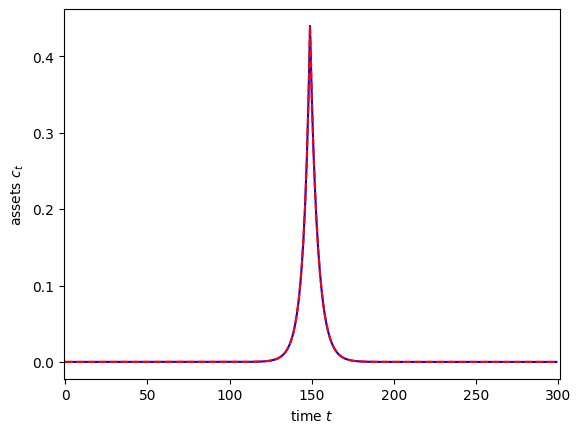
That looks like a tight match to me! As a second comparison exercise, let’s look at the impulse response of assets with respect to a change in permanent income risk in period \(s=150\). In this case, the shock variable is PermShkStd, but this parameter affects the constructed object IncShkDstn, so we will name that in construct.
NB: The proper SSJ calculator doesn’t require you to name constructed objects, but this “simpler” direct approach does. Why is that? It’s complicated and has to do with memory usage. We might improve this in the near future.
[13]:
t0 = time()
SSJ_K_sigma_psi = MyType.make_basic_SSJ(
    "PermShkStd",
    "aNrm",
    my_grid_specs,
    norm="PermShk",
    solved=True,
    offset=True,
)
t1 = time()
print("Constructing that SSJ took {:.3f}".format(t1 - t0) + " seconds in total.")
Constructing that SSJ took 5.862 seconds in total.
[14]:
t0 = time()
s = 150
dAds = MyType.calc_impulse_response_manually(
    "PermShkStd",
    "aNrm",
    my_grid_specs,
    s=s,
    norm="PermShk",
    construct=["IncShkDstn"],
    solved=True,
    offset=True,
)
t1 = time()
print(
    "Calculating that impulse response manually took {:.3f}".format(t1 - t0)
    + " seconds."
)
Calculating that impulse response manually took 5.697 seconds.
[15]:
plt.plot(dAds, "-b")
plt.plot(SSJ_K_sigma_psi[:, s], "--r")
plt.xlim(-1, 301)
plt.xlabel(r"time $t$")
plt.ylabel(r"assets $a_t$")
plt.show()
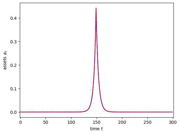
Hey, nailed it again! Note that calculating impulse responses for one particular period manually takes about the same time as building the entire SSJ matrix. That’s because (other than a bit of matrix arithmetic at the end) the bulk of the computation is the same, only the methodology for computing derivatives is different. This shows just how efficient the fake news algorithm is!