This page was generated from examples/Gentle-Intro/Gentle-Intro-To-HARK.ipynb.
Interactive online version: . Download notebook.

A Gentle Introduction to HARK

This notebook provides a simple, hands-on tutorial for first time HARK users – and potentially first time Python users. It does not go “into the weeds” - we have hidden some code cells that do boring things that you don’t need to digest on your first experience with HARK. Our aim is to convey a feel for how the toolkit works.

For readers for whom this is your very first experience with Python, we have put important Python concepts in boldface. For those for whom this is the first time they have used a Jupyter notebook, we have put Jupyter instructions in italics. Only cursory definitions (if any) are provided here. If you want to learn more, there are many online Python and Jupyter tutorials.

At the bottom of this notebook, we have included links to the other introductory notebooks for HARK.

# This cell has a bit of initial setup. You can click the triangle to the left to expand it.
# Click the "Run" button immediately above the notebook in order to execute the contents of any cell
# WARNING: Each cell in the notebook relies upon results generated by previous cells
#   The most common problem beginners have is to execute a cell before all its predecessors
#   If you do this, you can restart the kernel (see the "Kernel" menu above) and start over

from copy import deepcopy

mystr = lambda number: f"{number:.4f}"
import matplotlib.pyplot as plt
from HARK.utilities import plot_funcs

Your First HARK Model: Perfect Foresight

We start with almost the simplest possible consumption model: A consumer with CRRA utility

\begin{align*} U(C) = \frac{C^{1-\rho}}{1-\rho} \end{align*}

has perfect foresight about everything except the (stochastic) date of death, which may occur in each period, implying a “survival probability” each period of \(\newcommand{\LivPrb}{\mathsf{S}}\LivPrb_t \le 1\), and a complementary death probability of \(\mathsf{D}_t = 1 - \LivPrb_t\); death ends the consumer’s decision problem. Permanent labor income \(P_t\) grows from period to period by a factor \(\Gamma_t\). At the beginning of each period \(t\), the consumer has some amount of market resources \(M_t\) (which includes both market wealth and current income) and must choose how much of those resources to consume \(C_t\) and hold the rest in a riskless asset \(A_t\) which will earn return factor \(R\). The agent’s flow of utility \(U(C_t)\) from consumption is geometrically discounted by factor \(\beta\).

The agent’s problem can be written in Bellman form as:

\begin{align*} V_t(M_t,P_t) &= \max_{C_t}U(C_t) + \beta \LivPrb_t V_{t+1}(M_{t+1},P_{t+1})\\ &\text{s.t.} \\ A_t &= M_t - C_t \\ M_{t+1} &= R_{t+1} (M_{t}-C_{t}) + Y_{t+1}, \\ P_{t+1} &= \Gamma_{t+1} P_t, \\ \end{align*}

A particular perfect foresight agent’s problem can be characterized by values of risk aversion \(\rho\), discount factor \(\beta\), and return factor \(R\), along with sequences of income growth factors \(\{ \Gamma_t \}\) and survival probabilities \(\{\LivPrb\}\). To keep things simple, let’s forget about “sequences” of income growth and mortality, and just think about an infinite horizon consumer with constant income growth and survival probability: \(\Gamma_t = \Gamma\) and \(\LivPrb_t = \LivPrb\) for all \(t\).

Representing Agents in HARK

HARK represents agents solving this type of problem as \(\textbf{instances}\) of the \(\textbf{class}\) PerfForesightConsumerType, a \(\textbf{subclass}\) of AgentType. To make agents of this class, we must import the class itself into our workspace. (Run the cell below in order to do this).

from HARK.ConsumptionSaving.ConsIndShockModel import PerfForesightConsumerType

The PerfForesightConsumerType class contains within itself the Python code that constructs the solution for the perfect foresight model we are studying here, as specifically articulated in these lecture notes.

To create an instance of PerfForesightConsumerType, we simply call the class as if it were a function, passing as arguments the specific parameter values we want it to have. In the hidden cell below, we define a dictionary named PF_dictionary with these parameter values:

Param	Description	Code	Value
\(\rho\)	Relative risk aversion	CRRA	2.5
\(\beta\)	Discount factor	DiscFac	0.96
\(R\)	Risk free interest factor	Rfree	1.03
\(\LivPrb\)	Survival probability	LivPrb	0.98
\(\Gamma\)	Income growth factor	PermGroFac	1.01

For now, don’t worry about the specifics of dictionaries. All you need to know is that a dictionary lets us pass many arguments wrapped up in one simple data structure.

# This cell defines a parameter dictionary. You can expand it if you want to see what that looks like.
PF_dictionary = {
    "CRRA": 2.5,
    "DiscFac": 0.96,
    "Rfree": [1.03],
    "LivPrb": [0.98],
    "PermGroFac": [1.01],
    "cycles": 0,  # don't worry about this; it just means we want an infinite horizon model
}

Let’s make an object named PFexample which is an instance of the PerfForesightConsumerType class. The object PFexample will bundle together the abstract mathematical description of the solution embodied in PerfForesightConsumerType and the specific set of parameter values defined in PF_dictionary. Such a bundle is created by passing PF_dictionary to the class PerfForesightConsumerType:

PFexample = PerfForesightConsumerType(**PF_dictionary)
# The asterisks ** basically say "here come some arguments in a dictionary" to PerfForesightConsumerType.

In PFexample, we now have defined the problem of a particular infinite horizon perfect foresight consumer who knows how to solve this problem.

Note that each AgentType subclass has default parameters built right into it– you can make an instance of each class without passing any parameters at all!

Solving an Agent’s Problem

To tell the agent actually to solve the problem, we call the agent’s solve method. (A method is essentially a function that an object runs that affects the object’s own internal characteristics. In this case, the method adds the consumption function to the contents of PFexample.)

The cell below calls the solve method for PFexample.

PFexample.solve()

Running the solve method creates the attribute of PFexample named solution. In fact, every subclass of AgentType works the same way: The class definition contains the abstract algorithm that knows how to solve the model, but to obtain the particular solution for a specific instance (parameterization/configuration), that instance must be instructed to solve() its problem.

The solution attribute is always a list of solutions to a single period of the problem. In the case of an infinite horizon model like the one here, there is just one element in that list – the solution to all periods of the infinite horizon problem. The consumption function stored as the first element (index 0) of the solution list can be retrieved by:

PFexample.solution[0].cFunc

<HARK.interpolation.LinearInterp at 0x23986f991f0>

One of the results demonstrated in Chris Carroll’s lecture notes is that, for the specific problem defined above, there is a solution in which the ratio \(c = C/P\) is a linear function of the ratio of market resources to permanent income, \(m = M/P\).

This is why cFunc can be represented by a linear interpolation. It can be plotted between an \(m\) ratio of 0 and 10 using the command below.

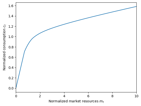
mPlotTop = 10
plt.xlabel(r"Normalized market resources $m_t$")
plt.ylabel(r"Normalized consumption $c_t$")
plot_funcs(PFexample.solution[0].cFunc, 0.0, mPlotTop)

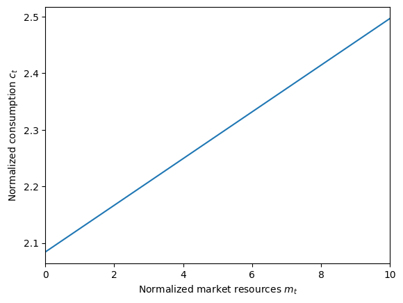
The figure illustrates one of the surprising features of the perfect foresight model: A person with zero money should be spending at a rate more than double their income (that is, cFunc(0.0) \(\approx 2.08\) - the intersection on the vertical axis). How can this be?

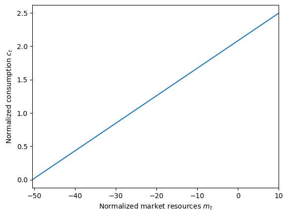
The answer is that we have not incorporated any constraint that would prevent the agent from borrowing against the entire PDV of future earnings– their “human wealth”. How much is that? What’s the minimum value of \(m_t\) where the consumption function is defined? We can check by retrieving the hNrm attribute of the solution, which calculates the value of human wealth normalized by permanent income:

humanWealth = PFexample.solution[0].hNrm
mMinimum = PFexample.solution[0].mNrmMin
print(
    "This agent's human wealth is "
    + str(humanWealth)
    + " times his current income level.",
)
print(
    "This agent's consumption function is defined (consumption is positive) down to m_t = "
    + str(mMinimum),
)

This agent's human wealth is 50.49994992551661 times his current income level.
This agent's consumption function is defined (consumption is positive) down to m_t = -50.49994992551661

Yikes! Let’s take a look at the bottom of the consumption function. In the cell below, the bounds of the plot_funcs function are set to display down to the lowest defined value of the consumption function.

plt.xlabel(r"Normalized market resources $m_t$")
plt.ylabel(r"Normalized consumption $c_t$")
plot_funcs(PFexample.solution[0].cFunc, mMinimum, mPlotTop)

Changing Agent Parameters

Suppose you wanted to change one (or more) of the parameters of the agent’s problem and see what that does. We want to compare consumption functions before and after we change parameters, so let’s make a new instance ofPerfForesightConsumerType by copying PFexample.

NewExample = deepcopy(PFexample)

You can assign new parameters to an AgentType with the assign_parameters method. For example, we could make the new agent less patient:

NewExample.assign_parameters(DiscFac=0.90)
NewExample.solve()
mPlotBottom = mMinimum
plt.xlabel(r"Normalized market resources $m_t$")
plt.ylabel(r"Normalized consumption $c_t$")
plot_funcs(
    [PFexample.solution[0].cFunc, NewExample.solution[0].cFunc],
    mPlotBottom,
    mPlotTop,
)

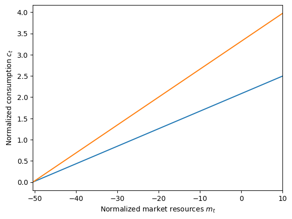
(Note that you can pass a list of functions to plot_funcs as the first argument rather than just a single function. Lists are written inside of [square brackets].)

Let’s try to deal with the “problem” of massive human wealth by making another consumer who has essentially no future income. We can virtually eliminate human wealth by making the permanent income growth factor very small.

In PFexample, the agent’s income grew by 1 percent per period – his PermGroFac took the value 1.01. What if our new agent had a growth factor of 0.01 – his income shrinks by 99 percent each period? In the cell below, set NewExample’s discount factor back to its original value, then set its PermGroFac attribute so that the growth factor is 0.01 each period.

Important: Recall that the model at the top of this document said that an agent’s problem is characterized by a sequence of income growth factors, but we tabled that concept. Because PerfForesightConsumerType treats PermGroFac as a time-varying attribute, it must be specified as a list (with a single element in this case).

# Revert NewExample's discount factor and make his future income minuscule
# WRITE YOUR CODE HERE!

# Compare the old and new consumption functions
plt.xlabel(r"Normalized market resources $m_t$")
plt.ylabel(r"Normalized consumption $c_t$")
plot_funcs([PFexample.solution[0].cFunc, NewExample.solution[0].cFunc], 0.0, 10.0)

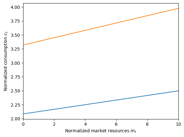
Now NewExample's consumption function has the same slope (MPC) asPFexample`, but it emanates from (almost) zero– he has basically no future income to borrow against!

If you’d like, use the cell above to alter NewExample’s other attributes (relative risk aversion CRRA, etc) and see how the consumption function changes. However, keep in mind that no solution exists for some combinations of parameters. HARK should let you know if this is the case if you try to solve such a model.

Your Second HARK Model: Adding Income Shocks

Linear consumption functions are pretty boring, and you’d be justified in feeling unimpressed if all HARK could do was plot some lines. Let’s look at another model that adds two important layers of complexity: income shocks and (artificial) borrowing constraints.

Specifically, our new type of consumer receives two income shocks at the beginning of each period: a completely transitory shock \(\theta_t\) and a completely permanent shock \(\psi_t\). Moreover, lenders will not let the agent borrow money such that his ratio of end-of-period assets \(A_t\) to permanent income \(P_t\) is less than \(\underline{a}\). As with the perfect foresight problem, this model can be framed in terms of normalized variables, e.g. \(m_t \equiv M_t/P_t\). (See here for all the theory). Accordingly, the normalized utility and continuation value are \(u\) and \(v_t\).

\begin{align*} v_t(m_t) &= \max_{c_t} u(c_t) + \LivPrb_t \beta \mathbb{E} [(\Gamma_{t+1}\psi_{t+1})^{1-\rho} v_{t+1}(m_{t+1}) ] ~~ \text{s.t.} \\ a_t &= m_t - c_t, \\ a_t &\geq \underline{a}, \\ m_{t+1} &= R_{t+1}/(\Gamma_{t+1} \psi_{t+1}) a_t + \theta_{t+1},\\ (\psi_{t+1},\theta_{t+1}) &\sim F_{t+1}, \\ \mathbb{E}[\psi_t]&=\mathbb{E}[\theta_t] = 1, \\ u(c) &= \frac{c^{1-\rho}}{1-\rho}. \end{align*}

HARK represents agents with this kind of problem as instances of the class IndShockConsumerType. To create an IndShockConsumerType, we must specify the same set of parameters as for a PerfForesightConsumerType, as well as an artificial borrowing constraint \(\underline{a}\) and a sequence of income shock distributions. It’s easy enough to pick a borrowing constraint – say, zero – but how would we specify the distributions of the shocks? Can’t the joint distribution of permanent and transitory shocks be just about anything?

Yes, and HARK can handle whatever correlation structure a user might care to specify. However, the default behavior of IndShockConsumerType is that the distribution of permanent income shocks is mean one lognormal, and the distribution of transitory shocks is mean one lognormal augmented with a point mass representing unemployment. The distributions are independent of each other by default, and by default are approximated with \(N\) point equiprobable distributions.

Let’s make an infinite horizon instance of IndShockConsumerType with the same parameters as our original perfect foresight agent, plus the extra parameters to specify the income shock distribution and the artificial borrowing constraint. As before, we’ll make a dictionary:

Param	Description	Code	Value
\(\underline{a}\)	Artificial borrowing constraint	BoroCnstArt	0.0
\(\sigma_\psi\)	Underlying stdev of permanent income shocks	PermShkStd	0.1
\(\sigma_\theta\)	Underlying stdev of transitory income shocks	TranShkStd	0.1
\(N_\psi\)	Number of discrete permanent income shocks	PermShkCount	7
\(N_\theta\)	Number of discrete transitory income shocks	TranShkCount	7
\(\mho\)	Unemployment probability	UnempPrb	0.05
\(\underset{\bar{}}{\theta}\)	Transitory shock when unemployed	IncUnemp	0.3

# This cell defines a parameter dictionary for making an instance of IndShockConsumerType.

IndShockDictionary = {
    "cycles": 0,
    "CRRA": 2.5,  # The dictionary includes our original parameters...
    "Rfree": [1.03],
    "DiscFac": 0.96,
    "LivPrb": [0.98],
    "PermGroFac": [1.01],
    "PermShkStd": [0.1],
    "PermShkCount": 7,  # and the new parameters for constructing the income process.
    "TranShkStd": [0.1],
    "TranShkCount": 7,
    "UnempPrb": 0.05,
    "IncUnemp": 0.3,
    "BoroCnstArt": 0.0,  # This says that the agent can't end the period with negative assets
}

As before, we need to import the relevant subclass of AgentType into our workspace, then create an instance by passing the dictionary to the class as if the class were a function.

from HARK.ConsumptionSaving.ConsIndShockModel import IndShockConsumerType

IndShockExample = IndShockConsumerType(**IndShockDictionary)

Now we can solve our new agent’s problem just like before, using the solve method.

IndShockExample.solve()
plt.xlabel(r"Normalized market resources $m_t$")
plt.ylabel(r"Normalized consumption $c_t$")
plot_funcs(IndShockExample.solution[0].cFunc, 0.0, 10.0)

This is a classic concave consumption function with risky labor income. We didn’t bother labeling axes for this simple example, but the horizontal axis represents normalized market resources \(m_t\) (cash-on-hand divided by permanent income) and the vertical axis represents normalized consumption.

Note that at low levels of \(m_t\), the slope of the consumption function is 1. This is where the agent is liquidity constrained: they want to consume more than their available \(m_t\), but are not permitted to because of the constrained that \(a_t \geq \underline{a} = 0\). Hence they consume as much as they can, \(c_t = m_t \longrightarrow a_t = 0\).

Changing Constructed Attributes

In the parameter dictionary above, we chose values for HARK to use when constructing its numeric representation of \(F_t\), the joint distribution of permanent and transitory income shocks. When IndShockExample was created, those parameters (TranShkStd, etc) were used by IndShockConsumerType to construct an attribute called IncomeDstn.

Suppose you were interested in changing (say) the amount of permanent income risk. From the section above, you might think that you could simply change the attribute TranShkStd, solve the model again, and it would work.

That’s almost true– there’s one small extra step. TranShkStd is a primitive input, but it’s not the thing you actually want to change. Changing TranShkStd doesn’t actually update the income distribution… unless you tell it to. Likewise, just like changing an agent’s preferences does not change the consumption function that was stored for the old set of parameters – until you invoke the solve method again). In the cell below, we invoke the method update so HARK knows to rebuild its constructed attributes, including IncomeDstn.

OtherExample = deepcopy(
    IndShockExample,
)  # Make a copy so we can compare consumption functions
OtherExample.assign_parameters(
    PermShkStd=[0.2],
)  # Double permanent income risk (note that it's a one element list)
OtherExample.update()  # Call the method to reconstruct the representation of F_t
OtherExample.solve()

In general, agents in HARK have an update method that calls all of their various constructors. If you change a parameter that describes a constructed attribute of your agent, invoking the update method will re-construct that attribute using the new parameter value.

You can learn more about constructors and model defaults in this notebook.

In the cell below, use your blossoming HARK skills to plot the consumption function for IndShockExample and OtherExample on the same figure.

# Use the line(s) below to plot the consumptions functions against each other

Learning More About HARK

This is the gentle introduction, giving you only the most basic information about how to use it… but there is so much more to cover!

Here is a set of links to additional introductory notebooks, organized by topic. We provide them here in our (loosely) suggested reading order, but they can mostly be tackled in any order you like.

• Simulation-Intro: Once you’ve solved a dynamic model, you probably want to see how the agents act out their model over time. This notebook provides an introduction to how simulation works in HARK.

• Cycles-Intro: Did you notice that we slipped the parameter cycles=0 into the dictionaries above, but then never discussed it? This notebook explains how HARK’s timing works, including both life-cycle and infinite horizon models… and more unusual cases.

• Constructors-Intro: We mentioned above that each AgentType subclass has default parameters, and that some model inputs are constructed. This notebook explains where default parameters and constructors live, and how to change constructors.

• Advanced-Intro: Assorted “advanced” concepts in HARK, including our distance metric, some uncommon solver options, utility functions, distribution objects, etc.

• Methods-Intro: This notebook explains some of the economic and numeric methods that we commonly use in HARK. This includes the endogenous grid method, interpolation methods, “pseudo-inverse” functions, and a discretization of the lognormal distribution.

• Model-List: Enough with all the explanations and details, just tell me about what models are in HARK! Ok, ok, here it is.

• AgentType-Intro: If you’re ready to not just use HARK’s models, but now make a new one on your own, this is the notebook you want to read. If you’re confused about something you found in our code and it seems to be a feature of AgentTypes generally, the answer is (hopefully) here.

• Market-Intro: AgentType is HARK’s superclass for “microeconomic” dynamic models, but we also have the Market superclass for “macroeconomic” models. This notebook explains why we put scare quotes on those terms, and how Market works.

• SSJ-tutorial: Most HARK AgentTypes are now capable of automatically generating sequence space Jacobians, which can be used with the sequence_jacobian toolkit. This notebook explains how that works (with examples).