Interactive online version:
Computing Heterogenous Agent Sequence Space Jacobians in HARK#
By William Du
This notebook illustrates how to compute Heterogenous Agent Sequence-Space Jacobian (HA-SSJ) matrices in HARK.
These matrices are a fundamental building building block to solving Heterogenous Agent New Keynesian Models with the sequence space jacobian methodology. For more information, see Auclert, Rognlie, Bardoszy, and Straub (2021)
We construct the HA-SSJs in two different ways. First, we make them using “handwritten” code that was specifically made for one particular model (the workhorse IndShockConsumerType). Second, we re-compute them using HARK’s new HA-SSJ constructor, which is meant to work with all of our AgentType subclasses. The figures below plot the results of both methods, but you might have to squint to see the difference between them!
[1]:
from time import time
import matplotlib.pyplot as plt

from HARK.ConsumptionSaving.ConsNewKeynesianModel import (
    NewKeynesianConsumerType,
)
from HARK.ConsumptionSaving.ConsIndShockModel import IndShockConsumerType
[2]:
# Define a simple function for plotting SSJs
def plot_SSJ(jacs, S, outcome, shock, T_max=None):
    colors = ["b", "r", "g", "m", "c"]
    if type(S) is int:
        S = [S]
    i = 0
    if T_max is None:
        if type(jacs) is list:
            T = jacs[0].shape[0]
        else:
            T = jacs.shape[0]
    else:
        T = T_max
    for s in S:
        c = colors[i]
        if type(jacs) is list:
            plt.plot(jacs[0][:, s], "-" + c, alpha=0.7, label="s=" + str(s))
            plt.plot(jacs[1][:, s], "--" + c)
        else:
            plt.plot(jacs[:, s], "-" + c, label="s=" + str(s))
        i += 1
    plt.legend()
    plt.xlabel(r"time $t$")
    plt.ylabel("rate of change of " + outcome)
    plt.title("SSJ for " + outcome + " with respect to " + shock + r" at time $s$")
    plt.tight_layout()
    plt.xlim(-1, T + 1)
    plt.show()


S_set = [0, 10, 30, 60, 100]  # list of s indices to plot
Create Agent#
[3]:
base_params = {
    "tolerance": 1e-12,
}

# Dictionary for IndShockConsumerType to match defaults of NewKeynesianConsumerType
alt_params = {
    "PermGroFac": [1.0],
    "aXtraMax": 50.0,
    "aXtraCount": 100,
    "DiscFac": 0.96,
    "tolerance": 1e-12,
    "cycles": 0,
}

swap_params = {
    "DiscFac": 0.94,
    "LivPrb": [0.9999],
}

# Turn this on to see what happens when we turn up survival and down discounting (offsetting)
if False:
    base_params.update(swap_params)
    alt_params.update(swap_params)

# Make a dictionary of grid specifications for the new version
assets_grid_spec = {"min": 0.0, "max": 50.0, "N": 301, "order": 3}
consumption_grid_spec = {"min": 0.0, "max": 3.0, "N": 901}
my_grid_specs = {"kNrm": assets_grid_spec, "cNrm": consumption_grid_spec}
[4]:
Agent = NewKeynesianConsumerType(**base_params)  # use mostly sdefault parameters
AltAgent = IndShockConsumerType(**alt_params)  # adjust to match defaults of ^^
Compute Steady State#
[5]:
start = time()
Agent.compute_steady_state()
print("Seconds to compute steady state by old method: {:.3f}".format(time() - start))
Seconds to compute steady state by old method: 11.358
Compute Jacobians#
Shocks possible with “handwritten” method: LivPrb, PermShkStd, TranShkStd, DiscFac, UnempPrb, Rfree, IncUnemp
Shock to Standard Deviation to Permanent Income Shocks#
[6]:
start = time()
CJAC_Perm, AJAC_Perm = Agent.calc_jacobian("PermShkStd", 300)
print("Seconds to calculate Jacobian by old method: {:.3f}".format(time() - start))
Seconds to calculate Jacobian by old method: 4.837
Do the same thing with the new version and compare them#
[7]:
# Compute the SSJs and time it
t0 = time()
SSJ_A_sigma_psi, SSJ_C_sigma_psi = AltAgent.make_basic_SSJ(
    "PermShkStd",
    ["aNrm", "cNrm"],
    my_grid_specs,
    norm="PermShk",
    offset=True,
)
t1 = time()
print(
    "Constructing those SSJs by the new method took {:.3f}".format(t1 - t0)
    + " seconds in total."
)
Constructing those SSJs by the new method took 13.223 seconds in total.
[8]:
plot_SSJ(
    [SSJ_C_sigma_psi, CJAC_Perm],
    S_set,
    "consumption",
    "stdev perm inc shocks",
    T_max=200,
)
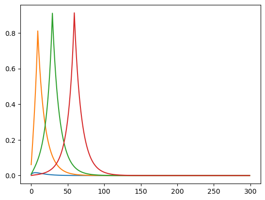
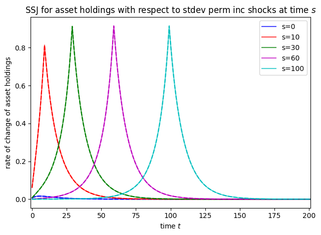
[9]:
plot_SSJ(
    [SSJ_A_sigma_psi, AJAC_Perm],
    S_set,
    "asset holdings",
    "stdev perm inc shocks",
    T_max=200,
)
Shock to Real Interest Rate#
[10]:
# Compute Jacobian using old method
start = time()
CJAC_Rfree, AJAC_Rfree = Agent.calc_jacobian("Rfree", 300)
print("Seconds to calculate Jacobian by old method: {:.3f}".format(time() - start))
Seconds to calculate Jacobian by old method: 4.619
Do the same thing with the new version and compare them#
[11]:
# Compute the SSJs and time it
t0 = time()
SSJ_A_r, SSJ_C_r = AltAgent.make_basic_SSJ(
    "Rfree",
    ["aNrm", "cNrm"],
    my_grid_specs,
    norm="PermShk",
    offset=True,
    solved=True,
)
t1 = time()
print("Constructing those SSJs took {:.3f}".format(t1 - t0) + " seconds in total.")
Constructing those SSJs took 6.786 seconds in total.
[12]:
plot_SSJ([SSJ_C_r, CJAC_Rfree], S_set, "consumption", "interest factor", T_max=200)
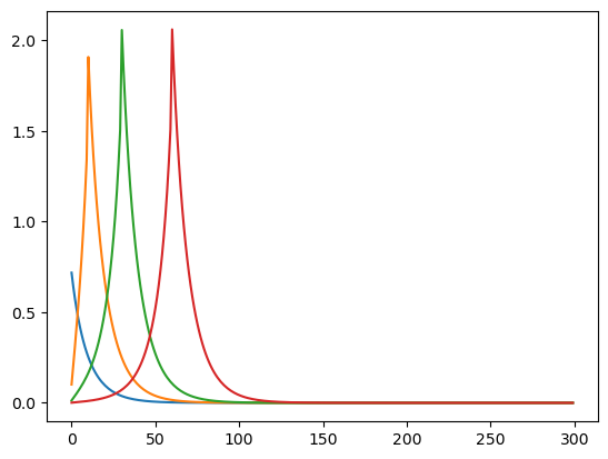
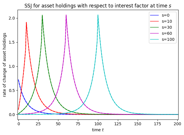
[13]:
plot_SSJ([SSJ_A_r, AJAC_Rfree], S_set, "asset holdings", "interest factor", T_max=200)
Shock to Unemployment Probability#
[14]:
# Make SSJs using old method
start = time()
CJAC_UnempPrb, AJAC_UnempPrb = Agent.calc_jacobian("UnempPrb", 300)
print("Seconds to calculate Jacobian by old method: {:.3f}".format(time() - start))
Seconds to calculate Jacobian by old method: 4.637
Do the same thing with the new version and compare them#
[15]:
# Compute the SSJs and time it
t0 = time()
SSJ_A_U, SSJ_C_U = AltAgent.make_basic_SSJ(
    "UnempPrb",
    ["aNrm", "cNrm"],
    my_grid_specs,
    norm="PermShk",
    offset=True,
    solved=True,
)
t1 = time()
print("Constructing those SSJs took {:.3f}".format(t1 - t0) + " seconds in total.")
Constructing those SSJs took 6.857 seconds in total.
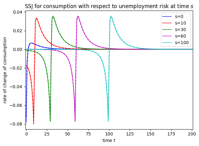
[16]:
plot_SSJ([SSJ_C_U, CJAC_UnempPrb], S_set, "consumption", "unemployment risk", T_max=200)
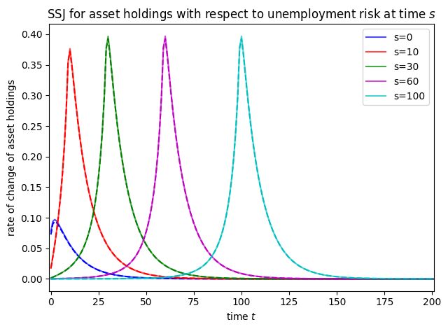
[17]:
plot_SSJ(
    [SSJ_A_U, AJAC_UnempPrb], S_set, "asset holdings", "unemployment risk", T_max=200
)
[ ]: