Interactive online version:
Solving Krusell Smith Model with HARK and SSJ#
By William Du
[1]:
import time

import matplotlib.pyplot as plt
import numpy as np
from scipy import optimize
from sequence_jacobian import create_model, simple  # functions
from sequence_jacobian.classes import JacobianDict, SteadyStateDict

from HARK.ConsumptionSaving.ConsNewKeynesianModel import NewKeynesianConsumerType
Calibration and setup#
This notebook uses the HARK toolkit to solve Krusell and Smith (1998), applying the Sequence Space Jacobian and SSJ toolkit.
Firm setup#
Collect calibration for the production economy in a dictionary.
[2]:
calibration = {
    "eis": 1,  # Elasticity of intertemporal substitution
    "delta": 0.025,  # Depreciation rate
    "alpha": 0.11,  # Capital share of income
    "L_ss": 1.0,  # Steady state labor
    "Y_ss": 1.0,  # Steady state output
    "r_ss": 0.01,  # Steady state real interest rate
}
Steady State Capital#
Find steady state capital (K_ss) and productivity (Z) implied by the firm’s first order condition, aggregate resource constraint and the above steady state values of labor (L_ss), the real interest rate (r_ss) and output (Y_ss).
[3]:
from scipy.optimize import root


def your_funcs(X):
    L_ss = calibration["L_ss"]
    alpha = calibration["alpha"]
    delta = calibration["delta"]
    r_ss = calibration["r_ss"]
    Y_ss = calibration["Y_ss"]

    K, Z = X

    # Firms first order condition and aggregate resource constraint
    f = [
        alpha * Z * (K / L_ss) ** (alpha - 1) - delta - r_ss,  # r_ss = MPK
        Z * K**alpha * L_ss ** (1 - alpha) - Y_ss,  # Y = Z*F(K,L)
    ]

    return f


sol = root(your_funcs, [1.0, 1.0])  # find roots

K_ss, Z_ss = sol.x

calibration["K_ss"] = K_ss
calibration["Z_ss"] = Z_ss
[4]:
print(sol)
 message: The solution converged.
 success: True
  status: 1
     fun: [ 1.749e-14 -5.218e-15]
       x: [ 3.143e+00  8.816e-01]
  method: hybr
    nfev: 14
    fjac: [[-3.675e-01  9.300e-01]
           [-9.300e-01 -3.675e-01]]
       r: [ 3.906e-02  1.143e+00 -3.236e-01]
     qtf: [-4.533e-12 -5.621e-12]
Double check the roots we find produce our chosen steady state values.
[5]:
def firm(
    K,
    Z,
    L_ss=calibration["L_ss"],
    alpha=calibration["alpha"],
    delta=calibration["delta"],
):
    r = alpha * Z * (K / L_ss) ** (alpha - 1) - delta
    w = (1 - alpha) * Z * (K / L_ss) ** alpha
    Y = Z * K**alpha * L_ss ** (1 - alpha)
    return r, w, Y


r_ss, w_ss, Y_ss = firm(sol.x[0], sol.x[1])

calibration["w_ss"] = w_ss
[6]:
print("--------------------------------------+------------")
print(f"Steady state capital                  | {K_ss:.4f}")
print(f"Steady state output                   | {Y_ss:.4f}")
print(f"Steady state real interest rate       | {r_ss:.4f}")
print(f"Steady state wage                     | {w_ss:.4f}")
print("--------------------------------------+------------")
--------------------------------------+------------
Steady state capital                  | 3.1429
Steady state output                   | 1.0000
Steady state real interest rate       | 0.0100
Steady state wage                     | 0.8900
--------------------------------------+------------
HARK agent#
HARK represents agent problems where aggregate variables can affect an individual income process as instances of NewKeynesianConsumerType, a subclass of AgentType (see A Gentle Introduction to HARK).
Instances of the NewKeynesianConsumerType class contain functions that solve policy functions of optimizing agents and compute Jacobian matrices in response to a policy shocks using the SSJ toolkit.
NOTE: NewKeynesianConsumerType is still a microeconomic agent solving an income fluctuation problem. The only difference from `IndShockConsumerType <https://docs.econ-ark.org/examples/HowWeSolveIndShockConsumerType/HowWeSolveIndShockConsumerType.html>`__ is that additional aggregate labour income variables are passed to the agent’s income process. This allows the agent’s problem to be defined within a general equilibrium framework such as (but not restricted to) HANK.
NOTE: Researchers can also create their own agent types by subclassing AgentType. See HARK’s documentation for more information.
To create an instance of NewKeynesianConsumerType, first specify parameters in a dictionary. To start, we use a discount factor of 0.98.
[7]:
L_ss = calibration["L_ss"]
w_ss = calibration["w_ss"]
r_ss = calibration["r_ss"]

HANK_Dict = {
    # Individual agent 'preferences' (shared with perfect foresight model)
    "CRRA": calibration["eis"],  # Coefficient of relative risk aversion
    "DiscFac": 0.98,  # Intertemporal discount factor
    "LivPrb": [0.99375],  # Survival probability
    # Individual lifcycle income process parameters
    "PermGroFac": [1.00],  # Permanent income growth factor
    "PermShkStd": [0.06],  # Standard deviation of log permanent shocks to income
    "PermShkCount": 5,  # Number of points in discrete approximation to permanent income shocks
    "TranShkStd": [0.2],  # Standard deviation of log transitory shocks to income
    "TranShkCount": 5,  # Number of points in discrete approximation to transitory income shocks
    # Parameters related to unemployment and retirement
    "UnempPrb": 0.0,  # Probability of unemployment while working
    "IncUnemp": 0.0,  # Unemployment benefits replacement rate
    "UnempPrbRet": 0.0000,  # Probability of "unemployment" while retired
    "IncUnempRet": 0.0,  # "Unemployment" benefits when retired
    "T_retire": 0.0,  # Period of retirement (0 --> no retirement)
    # Aggregates affecting the agent's decision
    "Rfree": [(1 + r_ss)],  # Interest factor for assets faced by agents
    "wage": [w_ss],  # Wage rate faced by agents
    "tax_rate": [
        0
    ],  # set to 0.0 because we are going to assume that labor here is actually after tax income
    "labor": [L_ss],  # Aggregate (mean) labor supply
    # Parameters for constructing "assets above minimum" grid
    "aXtraMin": 0.0001,  # Minimum end-of-period "assets above minimum" value
    "aXtraMax": 2000,  # Maximum end-of-period "assets above minimum" value
    "aXtraCount": 200,  # Number of points in the base grid of "assets above minimum"
    # Exponential nesting factor when constructing "assets above minimum" grid
    "aXtraNestFac": 3,
    "aXtraExtra": None,  # Additional values to add to aXtraGrid
    # Transition matrix simulation parameters
    "mCount": 200,
    "mMax": 2000,
    "mMin": 0.0001,
    "mFac": 3,
}
Let’s create a temporary instance of a NewKeynesianConsumerType agent.
[8]:
tempAgent = NewKeynesianConsumerType(**HANK_Dict)
Given a discount factor, the agent will supply a steady state capital stock A_ss.
[9]:
A_ss = tempAgent.compute_steady_state()[0]
print(f"Steady state agent asset supply for beta = 0.98 is: {A_ss:.3f}")
Steady state agent asset supply for beta = 0.98 is: 0.231
Steady State Assets#
Since we are interested in computing a steady state equilibrium, we find discFac such that A_ss clears the asset market given that K_ss is the steady state firm capital demand.
[10]:
def A_ss_func(beta):
    HANK_Dict["DiscFac"] = beta

    # For a given value of beta, we need to re-create the Agent
    Agent_func = NewKeynesianConsumerType(**HANK_Dict, verbose=False)

    # And then solve for the steady state supply
    A_ss = Agent_func.compute_steady_state()[0]

    return A_ss


def ss_dif(beta):
    return A_ss_func(beta) - Asset_target


start = time.time()
Asset_target = K_ss

DiscFac = optimize.brentq(ss_dif, 0.8, 0.9999)

print(f"Time taken to solve for steady state {time.time() - start:.3f} secs.")
Time taken to solve for steady state 11.408 secs.
We can now create the steady state agent using the general equilibrium discount factor.
[11]:
# Create a new agent
HANK_Dict["DiscFac"] = DiscFac
steadyHANK = NewKeynesianConsumerType(**HANK_Dict, verbose=False)
A_ss, C_ss = steadyHANK.compute_steady_state()
[12]:
# To make sure goods and asset markets clear
print(
    "Final goods clearing:",
    calibration["Y_ss"] - C_ss - calibration["delta"] * calibration["K_ss"],
)
print("Asset clearing:", A_ss - calibration["K_ss"])
Final goods clearing: 0.019151809710635556
Asset clearing: -4.28052704393167e-10
Computing Jacobians using SSJ#
With the steady state agent in hand, we can compute the Jacobians of the steady state HANK agent’s policy with respect to the aggregate state variables.
The calc_jacobian method of our NewKeynesianConsumerType agent computes the Jacobians of the steady state aggregate consumption (CJACW) and assets (AJACW) with respect to a pertubation of a specified variable.
Recall CJACW[s,t] is the time \(t\) response to a shock at time \(s\).
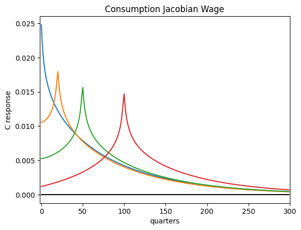
Here is an example where we shock the wage rate.
[13]:
start = time.time()

CJACW, AJACW = steadyHANK.calc_jacobian("wage", 300)  # Wage jacobians

print(f"Time taken to compute wage Jacobians: {time.time() - start:.3f} seconds")
Time taken to compute wage Jacobians: 4.084 seconds
[14]:
plt.plot(CJACW.T[0], label="s=0")
plt.plot(CJACW.T[20], label="s=20")
plt.plot(CJACW.T[50], label="s=50")
plt.plot(CJACW.T[100], label="s=100")
plt.xlim(-2, 300)
plt.plot(np.arange(300), np.zeros(300), color="k")
plt.title("Consumption Jacobian (Wage) ")
plt.xlabel("Quarters")
plt.ylabel("Consumption response")
plt.legend()
plt.show()
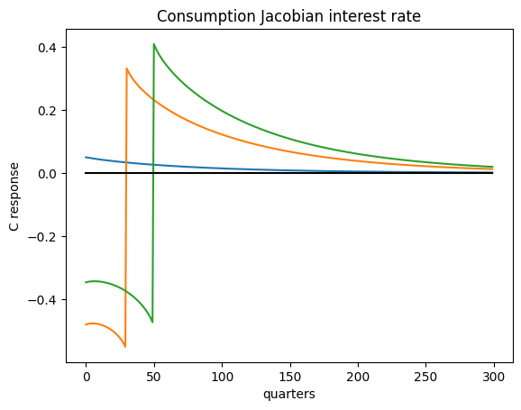
[15]:
start = time.time()

CJACR, AJACR = steadyHANK.calc_jacobian("Rfree", 300)  # Rfree jacobians

print(
    f"Time taken to compute return factor Jacobians: {time.time() - start:.3f} seconds"
)
Time taken to compute return factor Jacobians: 3.977 seconds
Here is an example where we shock the return factor.
[16]:
plt.plot(CJACR.T[0], label="s =0")
plt.plot(CJACR.T[20], label="s=20")
plt.plot(CJACR.T[50], label="s=50")
plt.plot(CJACR.T[100], label="s=100")
plt.plot(np.arange(300), np.zeros(300), color="k")
plt.title("Consumption Jacobian (Return Factor)")
plt.xlabel("Quarters")
plt.ylabel("Consumption response")
plt.show()
Let’s store the Jacobians in a dictionary for later use.
[17]:
# Store Jacobians in JacobianDict Object
Jacobian_Dict = JacobianDict(
    {
        "C": {
            "w": CJACW,
            "r": CJACR,
        },
        "A": {
            "w": AJACW,
            "r": AJACR,
        },
    },
)

# Construct SteadyStateDict object
SteadyState_Dict = SteadyStateDict(
    {
        "asset_mkt": 0.0,
        "goods_mkt": 0.0,
        "r": r_ss,
        "Y": Y_ss,
        "A": K_ss,
        "C": C_ss,
        "Z": Z_ss,
        "delta": calibration["delta"],
        "alpha": calibration["alpha"],
        "L": L_ss,
        "K": K_ss,
        "w": w_ss,
    },
)
Impulse Response Functions and Simulations#
[18]:
@simple
def firm(K, L, Z, alpha, delta):
    r = alpha * Z * (K(-1) / L) ** (alpha - 1) - delta
    w = (1 - alpha) * Z * (K(-1) / L) ** alpha
    Y = Z * K(-1) ** alpha * L ** (1 - alpha)
    return r, w, Y


@simple
def mkt_clearing(K, A, Y, C, delta):
    asset_mkt = A - K
    goods_mkt = Y - C - delta * K
    return asset_mkt, goods_mkt
[19]:
ks = create_model([Jacobian_Dict, firm, mkt_clearing], name="Krusell-Smith")
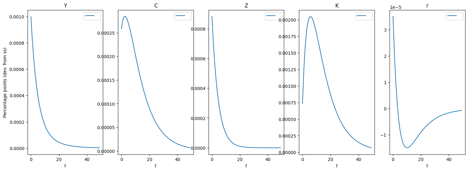
Solving for Impulse Responses#
[20]:
T = 300  # Length of the IRF
rho_Z = 0.8  # Persistence of IRF shock
dZ = 0.001 * Z_ss * rho_Z ** np.arange(T)
shocks = {"Z": dZ}

inputs = ["Z"]
unknowns = ["K"]
targets = ["asset_mkt"]

irfs_Z = ks.solve_impulse_linear(SteadyState_Dict, unknowns, targets, shocks)
[21]:
def show_irfs(
    irfs_list,
    variables,
    labels=[" "],
    ylabel=r"Percentage point (dev. from ss)",
    T_plot=50,
    figsize=(18, 6),
):
    if len(irfs_list) != len(labels):
        labels = [" "] * len(irfs_list)
    n_var = len(variables)
    fig, ax = plt.subplots(1, n_var, figsize=figsize, sharex=True)
    for i in range(n_var):
        # plot all irfs
        for j, irf in enumerate(irfs_list):
            ax[i].plot(irf[variables[i]][:50] * 1e2, label=labels[j])
        ax[i].set_title(variables[i])
        ax[i].set_xlabel(r"Quarters")
        if i == 0:
            ax[i].set_ylabel(ylabel)
        # ax[i].legend()
        # ax[i].x

    plt.tight_layout()
    plt.show()
    # plt.savefig("irf.png")
[22]:
# Impulse Responses to Productivity Shock
show_irfs([irfs_Z], ["Y", "C", "Z", "K", "r"])
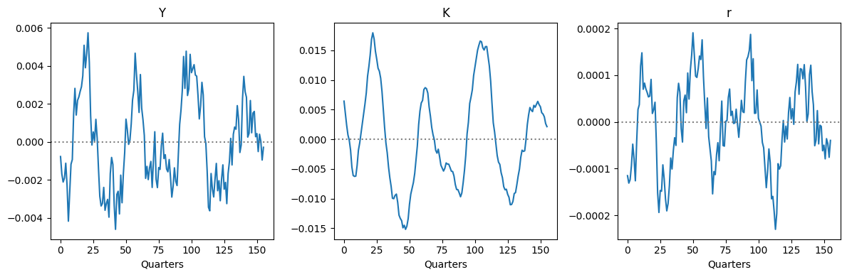
Simulating the model#
[23]:
from estimation.plots import plot_timeseries
from estimation.routines import simulate
[24]:
outputs = ["Y", "K", "r"]

sigmas = {"Z": 0.001}
rhos = {"Z": 0.8}
impulses = {}

for i in inputs:
    own_shock = {i: sigmas[i] * rhos[i] ** np.arange(T)}
    impulses[i] = ks.solve_impulse_linear(
        SteadyState_Dict,
        unknowns,
        targets,
        own_shock,
    )


T_sim = 156  # 39 years, as in the original SW (2007) sample
data_simul = simulate(list(impulses.values()), outputs, T_sim)
plot_timeseries(data_simul, (1, 3), figsize=(12, 4))