This page was generated from examples/ConsNewKeynesianModel/SSJ_explanation.ipynb.
Interactive online version: . Download notebook.

The Sequence Space Jacobian (SSJ) method

• Krusell and Smith (1997) solved their HA macro model with a “state space” method

  • They approximate the model solution for every conceivable combination of states

  • This is very expensive computationally

• The sequence space Jacobian method (SSJ) (Auclert et al., 2021) is an alternative

  • It computes a solution to the model for an expected path of shocks

  • This allows computation of the solution for only the interesting shocks

• The SSJ method solves for solutions to ‘MIT shocks’

  • The key requirement is that the MIT shocks be small, relative to the distribution of microeconomic state variables

  • This permits – in fact, requires – rich micro heterogeneity

  • SSJ is usable when there is an aggregate equilibrium and micro heterogeneity

    • So long as the “aggregate shocks” are relatively small

    • So it can be used to study industry or market equilibrium

• The algorithm assumes that agents have perfect foresight wrt aggregates

  • The model is deterministic wrt the evolution of aggregate “shocks”

• As a result, easily calculable Jacobian matrices are a “sufficient statistic”

  • They provide information sufficient to compute the macro dynamics

  • Even when the microfoundations have rich complexity and realism

Advantages of SSJ

• Can solve equilibrium models with rich microeconomic heterogeneity

  • Basic HANK models can take 3 seconds, previous methods take at least 15 minutes

• Can add additional exogenous aggregate shocks at virtually no cost.

Krusell Smith Model in Sequence Space

Here we solve a slightly simplified version of the Krusell-Smith model to clarify the exposition. In particular, we assume each household inelastically supplies \(\ell\) units of labor.

Households

Assume a continuum of atomistic households on the unit interval \([0,1]\) indexed by \(i\).

Assume households have perfect foresight over the real interest rate \(r_{t}\) and the real wage \(w_{t}\).

Household’s Problem

Households seek to maximize their expected discounted sum of lifetime utility of consumption. Variables that are idiosyncratic to a household have an \(i\) subscript, while aggregate variables do not.

\[V_{t}(m_{it}) = \max_{c_{it}} u(c_{it}) + E_{t}\left[ V_{t+1}(m_{it+1}) \right] \text{ s.t.}\]

\[m_{it} = y_{it} + (1+\mathit{r}_{t})k_{it-1},\]

\[c_{it} + k_{it}= m_{it},\]

\[k_{it} \geq 0,\]

where \(m_{it}\) is market resources (cash on hand), \(k_{it}\) is capital holdings and \(y_{it}\) is labor income.

Labor Income

Labor income is the product of an idiosyncratic transitory shock \(\theta\), the wage rate \(w\) (determined in aggregate), and the exogenously fixed individual labor supply \(\ell\):

\[y_{t} = \theta_{it} w_{t} \ell,\]

\[log(\theta_{it}) \sim N\left(-\frac{\sigma_{\theta}^2}{2}, \sigma_{\theta}^2 \right).\]

Firms and Production

Output is produced by firms via a Cobb-Douglas production function over aggregate capital \(K_t\) and labor \(L_t\), scaled by total factor productivity \(Z_t\):

\[Y_{t} = Z_{t}K_{t}^{\alpha}L_{t}^{1-\alpha}.\]

Determination of Wage and Interest Rates

Assume perfectly competitive markets, so that the factor prices are given by their marginal product:

\[w_{t} = (1-\alpha) Z_{t} K_{t}^{\alpha}L_{t}^{-\alpha},\]

\[r_{t} = \alpha Z_{t} K_{t}^{\alpha - 1} L_{t}^{1-\alpha}.\]

Dynamics of Productivity

TFP \(Z_t\) follows an AR(1) process in logs, with correlation factor \(\rho_Z\) and standard deviation of shocks \(\sigma_Z\).

\[log(Z_{t}) = \rho_{Z} \log( Z_{t-1}) + \epsilon_{t},\]

\[\epsilon_t \sim N(0, \sigma_Z^2).\]

Market Clearing

Aggregate capital and labor are found by aggregating idiosyncratic values over the population. For labor, this is trivial, as each household exogenously supplies \(\ell\) units of labor. To denote the switch to aggregate labor, apply a new label:

\[L_{t} = \int_0^1 \ell di = \ell \equiv \bar{L}.\]

Each household’s choice of capital holdings \(k_{it}\) depends on the entire future sequence of factor prices they will face. Denote that sequence as \(\left\{r_{s},w_{s}\right\}_{s=0}^{T}\), and the savings function in period \(t\) as \(\mathsf{k}_t(m_{it}, \cdot)\), which depends on current market resources and future prices. Then define aggregate capital as:

\[K_{t} = \int_{0}^{1} k_{it} di = \int_{0}^{1} \mathsf{k}_{t}(m_{it}, \left\{r_{s},w_{s}\right\}_{s=0}^{T}) di \equiv \mathcal{K}_{t}\left(\left\{r_{s},w_{s}\right\}_{s=0}^{T} \right).\]

Notice that aggregate capital \(K_t\) depends on the entire distribution of idiosyncratic market resources \(m_{it}\).

Model as defined by diff eqns in sequence space

The sequence-space equilibrium can be expressed as a root of a system of difference equations on the sequence of current and future prices and productivity shocks. For notational convenience, the sequence of aggregate outcomes will be represented by \(\textbf{U}\), and the sequence of productivity shocks by \(\textbf{Z}\). For period \(t\), the equilibrium conditions are:

\[\begin{split} H_{t}(\mathbf{U},\mathbf{Z}) = \begin{pmatrix} \mathcal{K}_{t}(\{r_{s} ,w_{s} \}_{s=t}^{s=T}) - K_{t} \\ \\ w_{t} - (1-\alpha) Z_{t} K_{t}^{\alpha} \bar{L}^{-\alpha} \\ \\ r_{t} - \alpha Z_{t} K_{t}^{\alpha - 1} \bar{L}^{1-\alpha} \\ \\ \end{pmatrix} = \begin{pmatrix} 0 \\ 0 \\ 0\\ \end{pmatrix} , \quad t=0,1,2,3,...\end{split}\]

where

\(\mathbf{U} = \left\{K_{t}, r_{t}, w_{t} \right\}_{t=0}^{s=T},\)

\(\mathbf{Z} = \left\{Z_{t}\right\}_{t=0}^{t=T}.\)

The equilibrium conditions for a single period can be stacked across all periods \(t=0,\cdots,T\), yielding the overall system:

\[\begin{split}\mathbf{H}(\mathbf{U},\mathbf{Z})= \begin{pmatrix} H_{0}(\mathbf{U},\mathbf{Z}) \\ \\ \vdots \\ \\ H_{t}(\mathbf{U},\mathbf{Z}) \\ \\ \vdots \\ \\ H_{T}(\mathbf{U},\mathbf{Z}) \\ \\ \end{pmatrix} = \begin{pmatrix} 0 \\ 0 \\ 0 \\ \vdots \\ 0 \\ 0 \\ 0 \\ \vdots \\ 0 \\ 0 \\ 0 \\ \end{pmatrix}.\end{split}\]

Solve the model by linearizing around the steady state

We are interested in how aggregate outcomes will change in response to exogenous shocks. Denote the endogenous impulse response as \(d\mathbf{U} \equiv \left\{dK_{t} , dr_{t} , dw_{t} \right\}_{t=0}^{t=T}\), and the exogenous shock (a change in future productivity shocks) as \(d\mathbf{Z} = \left\{ dZ_{t}\right\}_{t=0}^{t=T}\).

The characterization of the equilibrium conditions as a root of a system of equations \(\mathbf{H}(\mathbf{U},\mathbf{Z}) = 0\) defined on the sequence space allows us to apply the implicit function theorem to finf the impulse response:

\[d\mathbf{U} = -\mathbf{H}_{\mathbf{U}}(\mathbf{U}_{ss},\mathbf{Z}_{ss})^{-1} \mathbf{H}_{\mathbf{Z}}(\mathbf{U}_{ss},\mathbf{Z}_{ss}) d\mathbf{Z}.\]

We thus have a characterization of how aggregate outcomes respond to exogenous shocks near the steady state outcomes. In this context, the ``steady state productivity shock sequence’’ \(\mathbf{Z}_{ss}\) is simply \((0,\cdots,0)\), and the steady state outcome sequence is a constant sequence of aggregate capital and factor prices that obtain in the absence of macroeconomic shocks.

Heterogenous Agent Jacobian

When computing \(-\mathbf{H}_{\mathbf{U}}(\mathbf{U}_{ss},\mathbf{Z}_{ss})^{-1}\) we will need to compute the Jacobian of

\[\begin{split}\mathbf{F}(\mathbf{r},\mathbf{w}) = \begin{pmatrix} \mathcal{K}_{0}(\{r_{s}, w_{s} \}_{s=0}^{s=T})\\ \vdots \\ \mathcal{K}_{t}(\{r_{s} ,w_{s} \}_{s=0}^{s=T})\\ \vdots \\ \mathcal{K}_{T}(\{r_{s} ,w_{s} \}_{s=0}^{s=T})\\ \end{pmatrix}.\end{split}\]

More specifically, we will need the Jacobian matrices \(\mathbf{F}_{\mathbf{r}}(\mathbf{r},\mathbf{w})\) and \(\mathbf{F}_{\mathbf{w}}(\mathbf{r},\mathbf{w})\), where

\[\begin{split} \mathbf{F}_{\mathbf{r}}(\mathbf{r},\mathbf{w}) = \begin{pmatrix} \frac{ \partial \mathcal{K}_{0}}{\partial r_{0}} & ... & \frac{ \partial \mathcal{K}_{0}}{ \partial r_{t}} & ... & \frac{ \partial \mathcal{K}_{0}}{\partial r_{T}} \\ . \\ . \\ . \\ \frac{ \partial \mathcal{K}_{t}}{\partial r_{0}} & ... & \frac{ \partial \mathcal{K}_{t}}{ \partial r_{t}} & ... & \frac{ \partial \mathcal{K}_{t}}{\partial r_{T}} \\ . \\ . \\ . \\ \frac{ \partial \mathcal{K}_{T}}{\partial r_{0}} & ... & \frac{ \partial \mathcal{K}_{T}}{ \partial r_{t}} & ... & \frac{ \partial \mathcal{K}_{T}}{\partial r_{T}} \\ \\ \end{pmatrix}\end{split}\]

(and likewise for \(\mathbf{F}_{\mathbf{w}}(\mathbf{r},\mathbf{w})\)).

These Jacobian matrices are the most computationally complex object to compute in the model. On a 2024 laptop used to produce the results here, such methods can take up to 20 minutes for each matrix.

But the sequence space Jacobian methodology uses a ‘fake news’ algorithm to solve these matrices in under 3 seconds!

Overall algorithm

1. Define model in sequence space

\[\mathbf{H}(\mathbf{U},\mathbf{Z}) = \mathbf{0}\]

2. Solve for steady state

\[\mathbf{H}(\mathbf{U}_{ss},\mathbf{Z}_{ss}) = \mathbf{0}\]

where \(\mathbf{U}_{ss} = \left(U_{ss}, .. U_{ss}, .., U_{ss} \right)\)

3. Linearize around steady state and solve for impulse responses \(d\mathbf{U}\) given exogenous shock \(d\mathbf{Z}\)

\[d\mathbf{U} = -\mathbf{H}_{\mathbf{U}}^{-1} \mathbf{H}_{\mathbf{Z}} d\mathbf{Z}\]

When linearizing, find heterogenous agent Jacobians with fake news algorithm

What if the model contains many equations?

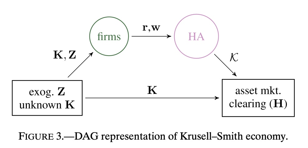
Here, because labor is exogenously supplied, aggregate capital \(K_t\) is a sufficient statistic for factor prices \(r_t\) and \(w_t\). The system above can thus be reduced to simply:

\[\begin{split}H_{t}(\mathbf{U},\mathbf{Z}) \equiv \begin{pmatrix} \mathcal{K}_{t}\left(\{\alpha Z_{t} K_{t}^{\alpha - 1} \bar{L}^{1-\alpha} ,(1-\alpha) Z_{s} K_{s}^{\alpha} \bar{L}^{-\alpha} \}_{s=0}^{s=T}\right) - K_{t} \\ \end{pmatrix} = 0, \quad t=0,1 ,2,3,....\end{split}\]

where \(\mathbf{U} = \left(K_{0},K_{1}.K_{2}....,K_{T} \right)\).

When the model contains many equations, we can represent the model as a directed acyclic graph to determine how the model should be reduced.

from IPython import display

display.Image("KS_DAG.jpeg")

Solving Using the HANK-SSJ Link

A companion notebook, KS-HARK-presentation presents the solution to the model described above using the HARK toolkit in combination with the SSJ toolkit.