This page was generated from examples/ConsIndShockModel/KinkedRconsumerType.ipynb.
Interactive online version: . Download notebook.

Higher Interest Rate to Borrow than Save

# Initial imports and notebook setup, click arrow to show

import matplotlib.pyplot as plt
import numpy as np
from time import time

from HARK.ConsumptionSaving.ConsIndShockModel import KinkedRconsumerType
from HARK.utilities import plot_funcs, plot_funcs_der

mystr = lambda number: f"{number:.4f}"

The module HARK.ConsumptionSaving.ConsIndShockModel concerns consumption-saving models with idiosyncratic shocks to (non-capital) income. All of the models assume CRRA utility with geometric discounting, no bequest motive, and income shocks are fully transitory or fully permanent.

ConsIndShockModel currently includes three models:

1. A very basic “perfect foresight” model with no uncertainty.

2. A model with risk over transitory and permanent income shocks.

3. The model described in (2), with an interest rate for debt that differs from the interest rate for savings.

This notebook provides documentation for the third of these models. \(\newcommand{\CRRA}{\rho}\) \(\newcommand{\DiePrb}{\mathsf{D}}\) \(\newcommand{\PermGroFac}{\Gamma}\) \(\newcommand{\Rfree}{\mathsf{R}}\) \(\newcommand{\DiscFac}{\beta}\)

Statement of “kinked R” model

Consider a small extension to the model faced by the IndShockConsumerType: that the interest rate on borrowing (\(a_t < 0\)) is greater than the interest rate on saving (\(a_t > 0\)). Consumers who face this kind of problem are represented by the KinkedRconsumerType class.

For a full theoretical treatment, this model analyzed in A Theory of the Consumption Function, With and Without Liquidity Constraints and its expanded edition.

Continuing to work with normalized variables (e.g. \(m_t\) represents the level of market resources divided by permanent income), the “kinked R” model can be stated as:

\begin{align*} v_t(m_t) &= \max_{c_t} u(c_t) + \DiscFac (1-\DiePrb_{t+1}) \mathbb{E}_{t} \left[(\PermGroFac_{t+1}\psi_{t+1})^{1-\CRRA} v_{t+1}(m_{t+1}) \right], \\ a_t &= m_t - c_t, \\ a_t &\geq \underline{a}, \\ m_{t+1} &= \Rfree_t/(\PermGroFac_{t+1} \psi_{t+1}) a_t + \theta_{t+1}, \\ \Rfree_t &= \begin{cases} \Rfree_{boro} & \text{if } a_t < 0\\ \Rfree_{save} & \text{if } a_t \geq 0, \end{cases}\\ \Rfree_{boro} &> \Rfree_{save}, \\ (\psi_{t+1},\theta_{t+1}) &\sim F_{t+1}, \\ \mathbb{E}[\psi]=\mathbb{E}[\theta] &= 1. \end{align*}

Solving the “kinked R” model

The solution method for the “kinked R” model is nearly identical to that of the IndShockConsumerType on which it is based, using the endogenous grid method; see the notebook for that model for more information. The only significant difference is that the interest factor varies by \(a_t\) across the exogenously chosen grid of end-of-period assets, with a discontinuity in \(\Rfree\) at \(a_t=0\).

To correctly handle this, the solveConsKinkedR function inserts two instances of \(a_t=0\) into the grid of \(a_t\) values: the first corresponding to \(\Rfree_{boro}\) (\(a_t = -0\)) and the other corresponding to \(\Rfree_{save}\) (\(a_t = +0\)). The two consumption levels (and corresponding endogenous \(m_t\) gridpoints) represent points at which the agent’s first order condition is satisfied at exactly \(a_t=0\) at the two different interest factors. 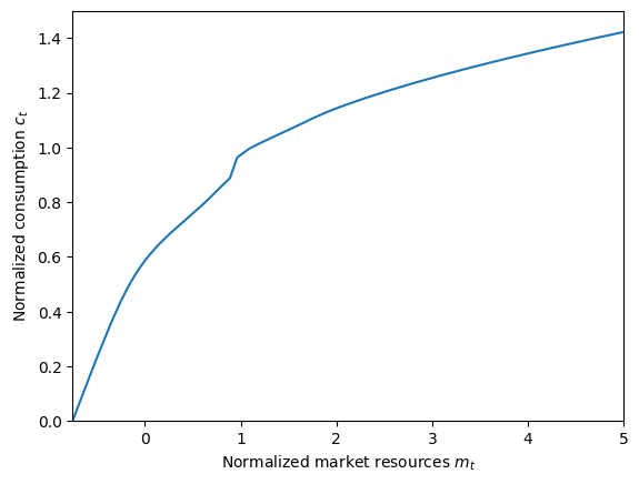In between these two points, the first order condition does not hold with equality: the consumer will end the period with exactly \(a_t=0\), consuming \(c_t=m_t\), but his marginal utility of consumption exceeds the marginal value of saving and is less than the marginal value of borrowing. This generates a consumption function with two kinks: two concave portions (for borrowing and saving) with a linear segment of slope 1 in between.

Example parameter values to construct an instance of KinkedRconsumerType

The parameters required to create an instance of KinkedRconsumerType are nearly identical to those for IndShockConsumerType. The only difference is that the parameter Rfree is replaced with Rboro and Rsave.

While the parameter \(\verb!CubicBool!\) is required to create a valid KinkedRconsumerType instance, it must be set to False; cubic spline interpolation has not yet been implemented for this model. In the future, this restriction will be lifted.

Parameter	Description	Code	Example value	Time-varying?
\(\DiscFac\)	Intertemporal discount factor	DiscFac	\(0.96\)
\(\CRRA\)	Coefficient of relative risk aversion	CRRA	\(2.0\)
\(\Rfree_{boro}\)	Risk free interest factor for borrowing	Rboro	\(1.20\)
\(\Rfree_{save}\)	Risk free interest factor for saving	Rsave	\(1.01\)
\(1 - \DiePrb_{t+1}\)	Survival probability	LivPrb	\([0.98]\)	\(\surd\)
\(\PermGroFac_{t+1}\)	Permanent income growth factor	PermGroFac	\([1.01]\)	\(\surd\)
\(\sigma_\psi\)	Standard deviation of log permanent income shocks	PermShkStd	\([0.1]\)	\(\surd\)
\(N_\psi\)	Number of discrete permanent income shocks	PermShkCount	\(7\)
\(\sigma_\theta\)	Standard deviation of log transitory income shocks	TranShkStd	\([0.2]\)	\(\surd\)
\(N_\theta\)	Number of discrete transitory income shocks	TranShkCount	\(7\)
\(\mho\)	Probability of being unemployed and getting \(\theta=\underline{\theta}\)	UnempPrb	\(0.05\)
\(\underline{\theta}\)	Transitory shock when unemployed	IncUnemp	\(0.3\)
\(\mho^{Ret}\)	Probability of being “unemployed” when retired	UnempPrbRet	\(0.0005\)
\(\underline{\theta}^{Ret}\)	Transitory shock when “unemployed” and retired	IncUnempRet	\(0.0\)
\((none)\)	Period of the lifecycle model when retirement begins	T_retire	\(0\)
\((none)\)	Minimum value in assets-above-minimum grid	aXtraMin	\(0.001\)
\((none)\)	Maximum value in assets-above-minimum grid	aXtraMax	\(20.0\)
\((none)\)	Number of points in base assets-above-minimum grid	aXtraCount	\(48\)
\((none)\)	Exponential nesting factor for base assets-above-minimum grid	aXtraNestFac	\(3\)
\((none)\)	Additional values to add to assets-above-minimum grid	aXtraExtra	\(None\)
\(\underline{a}\)	Artificial borrowing constraint (normalized)	BoroCnstArt	\(None\)
\((none)\)	Indicator for whether \(\verb!vFunc!\) should be computed	vFuncBool	\(True\)
\((none)\)	Indicator for whether \(\verb!cFunc!\) should use cubic splines	CubicBool	\(False\)

These example parameters are almost identical to those used for IndShockExample in the prior notebook, except that the interest rate on borrowing is 20% (like a credit card), and the interest rate on saving is 1%. Moreover, the artificial borrowing constraint has been set to None.

Solving and examining the solution of the “kinked R” model

The cell below creates an infinite horizon instance of KinkedRconsumerType and solves its model by calling its solve method.

KinkyExample = KinkedRconsumerType(cycles=0)  # default parameters, but infinite horizon
t0 = time()
KinkyExample.solve()
t1 = time()
print(
    "Solving the infinite horizon kinked R model took " + mystr(t1 - t0) + " seconds."
)

Solving the infinite horizon kinked R model took 0.0850 seconds.

An element of a KinkedRconsumerType’s solution will have all the same attributes as that of a IndShockConsumerType; see that notebook for details.

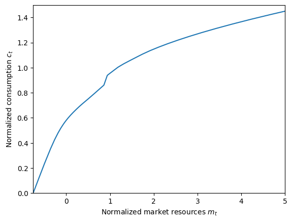
We can plot the consumption function of our “kinked R” example, as well as the MPC:

plt.xlabel(r"Normalized market resources $m_t$")
plt.ylabel(r"Normalized consumption $c_t$")
plt.ylim(0.0, 1.5)
plot_funcs(KinkyExample.solution[0].cFunc, KinkyExample.solution[0].mNrmMin, 5)

plt.xlabel(r"Normalized market resources $m_t$")
plt.ylabel(r"Marginal propensity to consume")
plt.ylim(0.0, 1.01)
plot_funcs_der(KinkyExample.solution[0].cFunc, KinkyExample.solution[0].mNrmMin, 5)

Simulating the “kinked R” model

In order to generate simulated data, an instance of KinkedRconsumerType needs to know how many agents there are that share these particular parameters (and are thus ex ante homogeneous), the distribution of states for newly “born” agents, and how many periods to simulated. These simulation parameters are described in the table below, along with example values.

Description	Code	Example value
Number of consumers of this type	AgentCount	\(10000\)
Number of periods to simulate	T_sim	\(500\)
Mean of initial log (normalized) assets	kLogInitMean	\(-6.0\)
Stdev of initial log (normalized) assets	kLogInitStd	\(1.0\)
Mean of initial log permanent income	pLogInitMean	\(0.0\)
Stdev of initial log permanent income	pLogInitStd	\(0.0\)
Aggregrate productivity growth factor	PermGroFacAgg	\(1.0\)
Age after which consumers are automatically killed	T_age	\(None\)

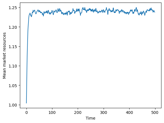
Here, we will simulate 10,000 consumers for 500 periods. All newly born agents will start with permanent income of exactly \(P_t = 1.0\), as pLvlInitStd has been set to zero; they will have essentially zero assets at birth, as kLogInitMean is \(-6.0\); assets will be less than \(1\%\) of permanent income at birth.

These example parameter values were already passed as part of the parameter dictionary that we used to create KinkyExample, so it is ready to simulate. We need to set the track_vars attribute to indicate the variables for which we want to record a history.

KinkyExample.track_vars = ["mNrm", "cNrm", "pLvl"]
KinkyExample.T_sim = 500
KinkyExample.initialize_sim()
KinkyExample.simulate()

We can plot the average (normalized) market resources in each simulated period:

plt.plot(np.mean(KinkyExample.history["mNrm"], axis=1))
plt.xlabel("Time")
plt.ylabel("Mean market resources")
plt.show()

Now let’s plot the distribution of (normalized) assets \(a_t\) for the current population, after simulating for \(500\) periods; this should be fairly close to the long run distribution:

plt.plot(
    np.sort(KinkyExample.state_now["aNrm"]),
    np.linspace(0.0, 1.0, KinkyExample.AgentCount),
)
plt.xlabel("End-of-period assets")
plt.ylabel("Cumulative distribution")
plt.ylim(-0.01, 1.01)
plt.show()

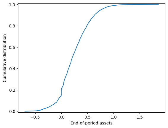
We can see there’s a significant point mass of consumers with exactly \(a_t=0\); these are consumers who do not find it worthwhile to give up a bit of consumption to begin saving (because \(\Rfree_{save}\) is too low), and also are not willing to finance additional consumption by borrowing (because \(\Rfree_{boro}\) is too high).

The smaller point masses in this distribution are due to HARK drawing simulated income shocks from the discretized distribution, rather than the “true” lognormal distributions of shocks. For consumers who ended \(t-1\) with \(a_{t-1}=0\) in assets, there are only 8 values the transitory shock \(\theta_{t}\) can take on, and thus only 8 values of \(m_t\) thus \(a_t\) they can achieve; the value of \(\psi_t\) is immaterial to \(m_t\) when \(a_{t-1}=0\). You can verify this by changing TranShkCount to some higher value, like 25, in the dictionary above, then running the subsequent cells; the smaller point masses will not be visible to the naked eye.