Interactive online version:
Representative Agent Models#
[1]:
from time import time

import numpy as np
import matplotlib.pyplot as plt

from HARK.ConsumptionSaving.ConsRepAgentModel import (
    RepAgentConsumerType,
    RepAgentMarkovConsumerType,
)
from HARK.utilities import plot_funcs
This module contains models for solving representative agent (RA) macroeconomic models. This stands in contrast to all other model modules in HARK, which (unsurprisingly) take a heterogeneous agents approach. In RA models, all attributes are either time invariant or exist on a short cycle. Also, models must be infinite horizon.
Representative Agent’s Problem#
Each period, the representative agent makes a decision about how much of his resources \(m_t\) he should consume \(c_t\) and how much should retain as assets \(a_t\). He gets a flow of utility from consumption, with CRRA preferences (with coefficient \(\rho\)). Retained assets are used to finance productive capital \(k_{t+1}\) in the next period. Output is produced according to a Cobb-Douglas production function using capital and labor \(\ell_{t+1}\), with a capital share of \(\alpha\); a fraction \(\delta\) of capital depreciates immediately after production.
The agent’s labor productivity is subject to permanent and transitory shocks, \(\psi_t\) and \(\theta_t\) respectively. The representative agent stands in for a continuum of identical households, so markets are assumed competitive: the factor returns to capital and income are the (net) marginal product of these inputs.
In the notation below, all lowercase state and control variables (\(m_t\), \(c_t\), etc) are normalized by the permanent labor productivity of the agent. The level of these variables at any time \(t\) can be recovered by multiplying by permanent labor productivity \(p_t\) (itself usually normalized to 1 at model start).
The agent’s problem can be written in Bellman form as:
\begin{eqnarray*} v_t(m_t) &=& \max_{c_t} U(c_t) + \beta \mathbb{E} [(\Gamma_{t+1}\psi_{t+1})^{1-\rho} v_{t+1}(m_{t+1})], \\ a_t &=& m_t - c_t, \\ \psi_{t+1} &\sim& F_{\psi t+1}, \qquad \mathbb{E} [F_{\psi t}] = 1,\\ \theta_{t+1} &\sim& F_{\theta t+1}, \\ k_{t+1} &=& a_t/(\Gamma_{t+1}\psi_{t+1}), \\ R_{t+1} &=& 1 - \delta + \alpha (k_{t+1}/\theta_{t+1})^{(\alpha - 1)}, \\ w_{t+1} &=& (1-\alpha) (k_{t+1}/\theta_{t+1})^\alpha, \\ m_{t+1} &=& R_{t+1} k_{t+1} + w_{t+1}\theta_{t+1}, \\ U(c) &=& \frac{c^{1-\rho}}{1-\rho} \end{eqnarray*}
The one period problem for this model is solved by the function solveConsRepAgent.
[2]:
# Make a quick example dictionary
RA_params = {
    "DeprRte": 0.05,
    "CapShare": 0.36,
    "UnempPrb": 0.0,
    "LivPrb": [1.0],
}
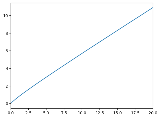
[3]:
# Make and solve a rep agent model
RAexample = RepAgentConsumerType(**RA_params)
t_start = time()
RAexample.solve()
t_end = time()
print(
    "Solving a representative agent problem took " + str(t_end - t_start) + " seconds.",
)

plt.ylim(0.0, 2.5)
plt.xlabel(r"Normalized market resources $m_t$")
plt.ylabel(r"Normalized consumption $c_t$")
plot_funcs(RAexample.solution[0].cFunc, 0, 20)
Solving a representative agent problem took 0.0910341739654541 seconds.
[4]:
# Simulate the representative agent model
RAexample.T_sim = 2000
RAexample.AgentCount = 1
RAexample.track_vars = ["cNrm", "mNrm", "Rfree", "wRte"]
RAexample.initialize_sim()
t_start = time()
RAexample.simulate()
t_end = time()
print(
    "Simulating a representative agent for "
    + str(RAexample.T_sim)
    + " periods took "
    + str(t_end - t_start)
    + " seconds.",
)
Simulating a representative agent for 2000 periods took 2.239887237548828 seconds.
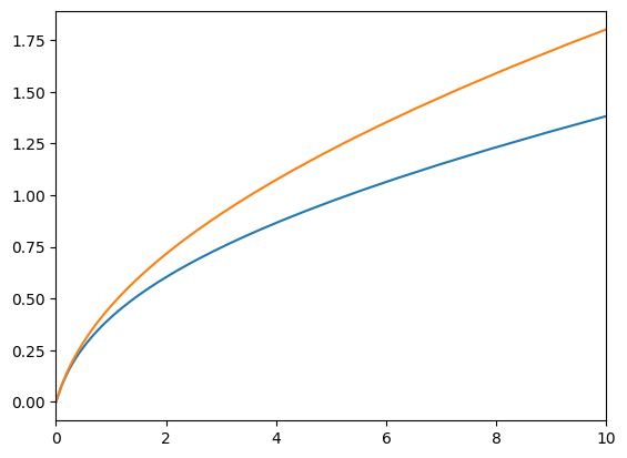
[5]:
# Make and solve a Markov representative agent
RA_markov_params = {
    "DeprRte": 0.05,
    "CapShare": 0.36,
    "UnempPrb": 0.0,
    "LivPrb": [1.0],
    "PermGroFac": [[0.97, 1.03]],
    "MrkvArray": np.array([[0.99, 0.01], [0.01, 0.99]]),
    "Mrkv": 0,
}
RAmarkovExample = RepAgentMarkovConsumerType(**RA_markov_params)
RAmarkovExample.IncShkDstn = [2 * [RAmarkovExample.IncShkDstn[0]]]
t_start = time()
RAmarkovExample.solve()
t_end = time()
print(
    "Solving a two state representative agent problem took "
    + str(t_end - t_start)
    + " seconds.",
)

plt.ylim(0.0, 3.0)
plt.xlabel(r"Normalized market resources $m_t$")
plt.ylabel(r"Normalized consumption $c_t$")
plot_funcs(RAmarkovExample.solution[0].cFunc, 0, 20)
Solving a two state representative agent problem took 0.2400679588317871 seconds.
[6]:
# Simulate the two state representative agent model
RAmarkovExample.T_sim = 2000
RAmarkovExample.AgentCount = 1
RAmarkovExample.track_vars = ["cNrm", "mNrm", "Rfree", "wRte", "Mrkv"]
RAmarkovExample.initialize_sim()
t_start = time()
RAmarkovExample.simulate()
t_end = time()
print(
    "Simulating a two state representative agent for "
    + str(RAexample.T_sim)
    + " periods took "
    + str(t_end - t_start)
    + " seconds.",
)
Simulating a two state representative agent for 2000 periods took 2.315621852874756 seconds.