This page was generated from examples/ConsWealthUtilityModel/CapitalistSpiritConsumerType.ipynb.
Interactive online version: . Download notebook.

Wealth-in-Utility Additively with Consumption

The typical consumption-saving model assumes that agents derive a flow of utility from consumption each period, with additively separable utility across time. In HARK.ConsumptionSaving.ConsWealthUtility module, we change this assumption to allow wealth (end-of-period assets) to enter the agent’s utility function directly.

This notebook concerns agents whose direct preferences for wealth are represented additively with consumption utility as a second CRRA term. For multiplicative direct preferences for wealth, see the notebook for ``WealthUtilityConsumerType` <./WealthUtilityConsumerType.ipynb>`__ in the same module. The name of the AgentType subclass, and the model itself, is based on Johanna Francis’ paper “Wealth and the Capitalist Spirit”.

# Import basic tools and our AgentType of interest
import numpy as np
import matplotlib.pyplot as plt
from time import time
from HARK.utilities import plot_funcs
from HARK.ConsumptionSaving.ConsWealthUtilityModel import CapitalistSpiritConsumerType

Additive Wealth-in-Utility Consumption-Saving Model Statement

A CapitalistSpiritConsumerType’s problem can be expressed as:

\(\newcommand{\R}{\mathbb{R}}\) \(\newcommand{\CRRA}{\rho}\) \(\newcommand{\LivPrb}{\mathsf{S}}\) \(\newcommand{\PermGroFac}{\Gamma}\) \(\newcommand{\Rfree}{\mathsf{R}}\) \(\newcommand{\DiscFac}{\beta}\) \(\newcommand{\CRRAwealth}{\nu}\) \(\newcommand{\WealthCurve}{\hat{\CRRAwealth}}\) \(\newcommand{\WealthFac}{\alpha}\) \(\newcommand{\WealthShift}{\xi}\) \(\newcommand{\cLvl}{C}\) \(\newcommand{\mLvl}{M}\) \(\newcommand{\aLvl}{A}\)

\begin{eqnarray*} V_t(\mLvl_t,p_t) &=& \max_{\cLvl_t} ~~ U(\cLvl_t, \aLvl_t) + \beta \LivPrb_t \mathbb{E}_{t} [v_{t+1}(\mLvl_{t+1}, p_{t+1})] ~~ \text{s.t.}\\ \aLvl_t &=& \mLvl_t - \cLvl_t, \\ \aLvl_t &\geq& \underline{a} \cdot p_t, \\ \mLvl_{t+1} &=& \Rfree \aLvl_t + \theta_{t+1}, \\ p_{t+1} &=& G_{t+1}(p_t)\psi_{t+1}, \\ \psi_t \sim F_{\psi_t} &\qquad& \theta_t \sim F_{\theta_t}, \\ \mathbb{E} [F_{\psi_t}] &=& 1, \\ U(\cLvl, \aLvl) &=& \frac{\cLvl^{1-\CRRA}}{1-\CRRA} + \WealthFac \frac{(\aLvl + \WealthShift)^{1-\CRRAwealth}}{1-\CRRAwealth}, ~~~ \CRRAwealth = \CRRA \cdot \WealthCurve. \end{eqnarray*}

This model is identical to that of `GenIncProcessConsumerType <../ConsGenIncProcessModel/GenIncProcessConsumerType.ipynb>`__ except for an addition to the utility function, which now depends on both consumption \(\cLvl_t\) and end-of-period wealth \(\aLvl_t\).

In the “capitalist spirit” model, wealth enters utility directly as a second CRRA term, additive with utility of consumption. This term has a risk aversion coefficient of \(\CRRAwealth < \CRRA\) (or more precisely \(\WealthCurve \in (0,1)\)), which generates luxury preferences for wealth accumulation: wealthier agents want to acquire even more wealth, and the saving rate will tend toward 100% as wealth becomes arbitrarily large.

Solving the Additive Wealth-in-Utility Model

Whereas the WealthUtilityConsumerType was represented with a permanent-income-normalized problem, building from the workhorse IndShockConsumerType, the CapitalistSpiritConsumerType’s model is not normalized by permanent income. Indeed, the intent of this model is that preferences are not homothetic with respect to income, and richer agents will want to accumulate (proportionally) more wealth.

Luckily, this model is actually much more straightforward to solve than the WealthUtilityConsumerType model. Following the EGM logic used throughout HARK, define end-of-period (or continuation) value as:

\begin{equation*} \mathfrak{V}_t(\aLvl_t, p_t) \equiv \beta \LivPrb_t \mathbb{E}_{t} [V_{t+1}(\Rfree \aLvl_t + \theta_{t+1}, G_{t+1}(p_t)\psi_{t+1})]. \end{equation*}

Likewise, end-of-period marginal value of assets is:

\begin{equation*} \mathfrak{V}^\aLvl_t(\aLvl_t, p_t) \equiv \beta \Rfree \LivPrb_t \mathbb{E}_{t} [V^\mLvl_{t+1}(R \aLvl_t + \theta_{t+1}, G_{t+1}(p_t)\psi_{t+1})]. \end{equation*}

The first order condition for optimal consumption can then be expressed in EGM form as:

\begin{equation*} \cLvl_t^{-\CRRA} - \WealthFac (\aLvl_t + \WealthShift)^{-\CRRAwealth} - \mathfrak{V}^\aLvl_t(\aLvl_t, p_t) = 0 \Longrightarrow \cLvl_t = \left( \WealthFac (\aLvl_t + \WealthShift)^{-\CRRAwealth} + \mathfrak{V}^\aLvl_t(\aLvl_t, p_t) \right)^{-1/\CRRA}. \end{equation*}

Thus the “capitalist spirit” model is barely more complex to solve than its parent GenIncProcessModel– just an additional closed form term is added to the marginal value of wealth before applying the inverse marginal utility function. More broadly, GenIncProcess is the “capitalist spirit” model with \(\WealthFac = 0\)– the agent puts zero relative utility weight on their assets.

The remainder of the solution method proceeds as usual for HARK and EGM, so we won’t further elaborate on it here.

Example Parameter Values to Make a CapitalistSpiritConsumerType

Most of the parameters and objects required to specify and solve a CapitalistSpiritConsumerType are shared with the GenIncProcessConsumerType, with only a few simple parameters added.

Param	Description	Code	Value	Constructed
\(\DiscFac\)	Intertemporal discount factor	DiscFac	0.96
\(\CRRA\)	Coefficient of relative risk aversion	CRRA	2.0
\(\WealthFac\)	Scaling factor for relative preference for wealth	WealthFac	1.0
\(\WealthCurve\)	Risk aversion for wealth as compared to consumption (must be in \((0,1)\))	WealthCurve	0.8
\(\WealthShift\)	Additive shifter for wealth in utility function	WealthShift	4.0
\(\Rfree_t\)	Risk free interest factor	Rfree	[1.03]
\(\LivPrb_t\)	Survival probability	LivPrb	[0.98]
\(\underline{a}\)	Artificial borrowing constraint, as factor of permanent income	BoroCnstArt	0.0
\((none)\)	Indicator for whether vFunc should be computed	vFuncBool	True
\((none)\)	Indicator for whether cFunc should use cubic splines	CubicBool	False
\(F_t\)	Joint distribution of permanent and transitory income shocks	IncomeDstn		\(\surd\)
\(G_t\)	Expected persistent income next period as a function of this period’s level	pLvlNextFunc		\(\surd\)
\((none)\)	Array of persistent income levels	pLvlGrid		\(\surd\)
\((none)\)	Array of end-of-period assets above minimum	aXtraGrid		\(\surd\)

Constructed Inputs for CapitalistSpiritConsumerType

The default constructors for CapitalistSpiritConsumerType are identical to those for PersistentShockConsumerType:

• IncShkDstn is constructed with construct_lognormal_income_process_unemployment, using parameters like PermShkStd, PermShkCount, TranShkStd, TranShkCount, IncUnemp, and UnempPrb. This is the standard income shock distribution constructor throughout HARK.

• aXtraGrid is constructed with make_assets_grid, as in most other HARK models, and represents normalized asset levels; i.e. it is rescaled by permanent income for each \(p_t\) in pLvlGrid when solving the model

• pLvlNextFunc is constructed with make_AR1_style_pLvlNextFunc, with a default persistence coefficient of 0.98. Thus persistent income follows an AR(1) in logs, as for a PersistentShockConsumerType. When cycles=1, PermGroFac can be any life-cycle sequences of expected growth factors. When cycles=0, the model will only behave as expected when PermGroFac=1.0.

• pLvlGrid is constructed with make_pLvlGrid_by_simulation, which literally simulates a large number of \(p_t\) sequences using pLvlNextFunc, IncShkDstn, and the initial distribution of permanent income specified in pLvlInitDstn. It then builds the (age-conditional) grid of persistent income levels based on the specified pLvlPctiles. Just as in PersistentShockConsumerType, this function is only compatible with cycles=0 (infinite horizon) and cycles=1 (lifecycle model).

Example Implementations of CapitalistSpiritConsumerType

The default parameters for CapitalistSpiritConsumerType are fairly sensible and mostly copied from GenIncProcessConsumerType. Let’s make an infinite horizon instance with otherwise default parameters, but increase income persistence to 99% from its default 98% (to increase the spread of permanent income levels).

For the parameters novel to this model, the defaults are WealthFac = 1.0, WealthCurve = 0.8, and WealthShift = 0.0. With default CRRA = 2.0, that means that \(\CRRAwealth = 1.6\) by default for this AgentType subclass.

Just like for PersistentShockConsumerType, instantiating an infinite horizon CapitalistSpiritConsumerType takes a few seconds because the pLvlGrid is constructed by simulation over many periods.

def mystr(x):
    return "{:.4f}".format(x)

# Make an infinite horizon capitalist spirit type with otherwise default parameters
t0 = time()
SpiritType = CapitalistSpiritConsumerType(cycles=0, PrstIncCorr=0.99)
t1 = time()
print(
    "Instantiating an infinite horizon capitalist spirit consumer type took "
    + mystr(t1 - t0)
    + " seconds."
)

Instantiating an infinite horizon capitalist spirit consumer type took 7.3447 seconds.

# Solve the infinite horizon model
t0 = time()
SpiritType.solve()
t1 = time()
print(
    "Solving an infinite horizon capitalist spirit consumer type took "
    + mystr(t1 - t0)
    + " seconds."
)

Solving an infinite horizon capitalist spirit consumer type took 13.4974 seconds.

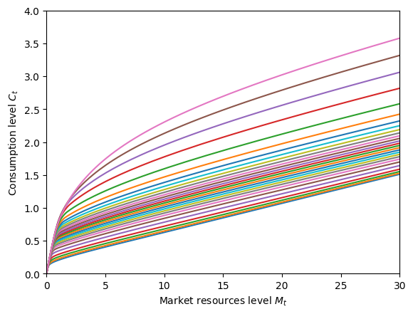
Like for other AgentType subclasses, let’s plot the consumption function. For this model, we will plot it at each of the permanent income levels in pLvlGrid.

# Plot the consumption function by pLvl
SpiritType.unpack("cFunc")
plt.ylim(0.0, 4.0)
plt.xlabel(r"Market resources level $M_t$")
plt.ylabel(r"Consumption level $C_t$")
plot_funcs(SpiritType.cFunc[0].functions[0].func.xInterpolators, 0.0, 30.0)

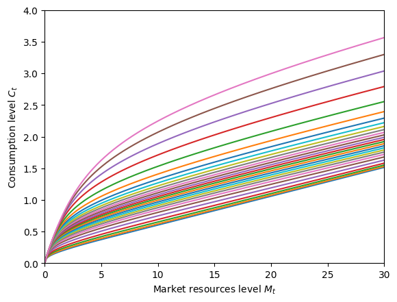
Even though this agent is guaranteed to have positive income each period (under default parameters) and is liquidity constrained, they never choose to end the period with \(A_t = 0\) in wealth, because this would yield negative infinite utility given their preferences.

To see how preferences are non-homothetic in this model, let’s plot the permanent income normalized consumption functions. Because wealth accumulation is a luxury good, we should expect to see higher income agents consume less conditional on their market resources to permanent income ratio.

# Plot the normalized consumption functions by pLvl
pLvlGrid = SpiritType.pLvlGrid[0]
mNrm = np.linspace(0.0, 50.0, 301)
for j in range(pLvlGrid.size):
    pLvl = pLvlGrid[j]
    mLvl = pLvl * mNrm
    cLvl = SpiritType.cFunc[0].functions[0].func.xInterpolators[j](mLvl)
    cNrm = cLvl / pLvl
    plt.plot(mNrm, cNrm)
plt.ylim(0.0, 4.0)
plt.xlim(0.0, 50.0)
plt.xlabel(r"Normalized market resources $m_t$")
plt.ylabel(r"Normalized consumption $c_t$")
plt.show()

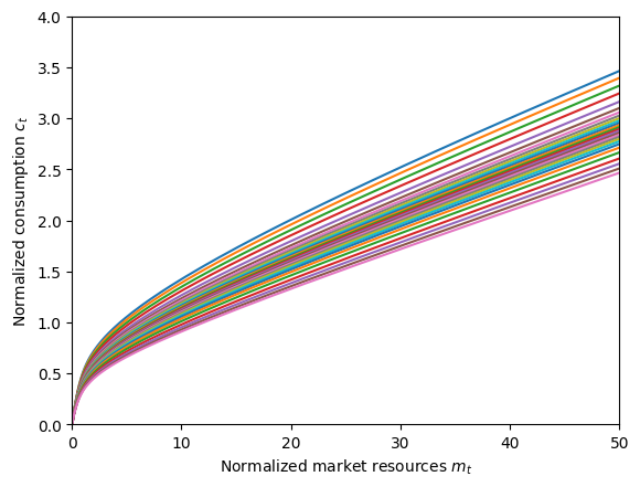
As expected, the highest permanent income level (pink) consumes the least relative to their normalized market resources. This is somewhat a product of permanent income being expected to fall for the richest agents and rise for the poorest, but the direct preference for wealth is a much larger contributor.

To see this, we can make the luxury effect of wealth even stronger by reducing WealthCurve from its default of 0.8 and resolving the model.

# Make and solve a capitalist spirit type that puts even more weight on wealth as they become richer
t0 = time()
LuxuryType = CapitalistSpiritConsumerType(
    cycles=0, WealthCurve=0.4, aXtraMax=150.0, aXtraCount=200
)
LuxuryType.solve()
t1 = time()
print("Making and solving that kind of agent took " + mystr(t1 - t0) + " seconds.")

Making and solving that kind of agent took 50.6384 seconds.

# Plot the normalized consumption functions by pLvl
LuxuryType.unpack("cFunc")
pLvlGrid = LuxuryType.pLvlGrid[0]
mNrm = np.linspace(0.0, 50.0, 301)
for j in range(pLvlGrid.size):
    pLvl = pLvlGrid[j]
    mLvl = pLvl * mNrm
    cLvl = LuxuryType.cFunc[0].functions[0].func.xInterpolators[j](mLvl)
    cNrm = cLvl / pLvl
    plt.plot(mNrm, cNrm)
plt.ylim(0.0, 4.0)
plt.xlim(0.0, 50.0)
plt.xlabel(r"Normalized market resources $m_t$")
plt.ylabel(r"Normalized consumption $c_t$")
plt.show()

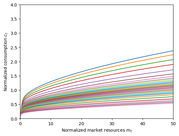
Now you can really see the extreme dispersion in normalized consumption by permanent income level. A lower value of WealthCurve means that the CRRA for wealth \(\CRRAwealth\) is lower compared to ordinary \(\CRRA\). That means it has less curvature, so the marginal utility of wealth decreases slower than the marginal utility of consumption. Hence as consumption and wealth increase, the agent increasingly gets relatively more marginal utility from wealth than consumption, and they want to save even more than they already have.

Note that even though normalized consumption is lower for higher income agents (conditional on normalized) market resources, higher income consumers still consume more in level conditional on market resources level. Let’s plot the non-normalized consumption functions to see that:

# Plot the consumption function by pLvl
plt.ylim(0.0, 1.5)
plt.xlabel(r"Market resources level $M_t$")
plt.ylabel(r"Consumption level $C_t$")
plot_funcs(LuxuryType.cFunc[0].functions[0].func.xInterpolators, 0.0, 30.0)

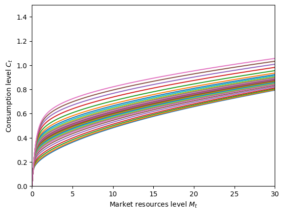
Note that we increased the upper bound of the aXtraGrid for this example. That’s because we didn’t want this figure to contradict our economic claim that consumption level is still increasing in \(p_t\), holding \(M_t\) fixed. Because the lowest value of \(p_t\) in the pLvlGrid is so low, the consumption function at the lowest \(p_t\) would overtake the consumption function elsewhere due to linear extrapolation.

In fact, if you simply increase the plotting boundaries of this figure, you’ll get the consumption function to “flip” or “twist”. This is just a product of linear extrapolation kicking in at different market resource levels by \(p_t\), not a true feature of the consumption function!

Finally, let’s look at the role of the WealthShift parameter, which is zero by default. If it is instead positive, then agents do not get negative infinte utility from ending the period with \(A_t = 0\), and they will be willing to do so at low levels of market resources. This will make the luxury effect of wealth become active at higher wealth levels.

# Make a capitalist spirit consumer type with positive `WealthShift`
t0 = time()
ShiftType = CapitalistSpiritConsumerType(cycles=0, WealthShift=2.0, PrstIncCorr=0.99)
ShiftType.solve()
t1 = time()
print("Making and solving that agent took " + mystr(t1 - t0) + " seconds.")

Making and solving that agent took 20.0935 seconds.

# Plot the consumption function by pLvl
ShiftType.unpack("cFunc")
plt.ylim(0.0, 4.0)
plt.xlabel(r"Market resources level $M_t$")
plt.ylabel(r"Consumption level $C_t$")
plot_funcs(ShiftType.cFunc[0].functions[0].func.xInterpolators, 0.0, 30.0)

Compare that consumption function to the very first one in this notebook and you’ll see that the agent is more willing to consume at low levels of market resources.