This page was generated from examples/ConsBequestModel/example_WarmGlowBequest.ipynb.
Interactive online version: . Download notebook.

Warm-Glow Bequest Motive

This notebook only provides examples, without explaining the model. It will be revised and improved in the near future.

from copy import copy
from time import time

import matplotlib.pyplot as plt
import pandas as pd

from HARK.Calibration.Income.IncomeTools import (
    CGM_income,
    parse_income_spec,
    parse_time_params,
)
from HARK.Calibration.life_tables.us_ssa.SSATools import parse_ssa_life_table
from HARK.Calibration.SCF.WealthIncomeDist.SCFDistTools import (
    income_wealth_dists_from_scf,
)
from HARK.ConsumptionSaving.ConsBequestModel import (
    BequestWarmGlowConsumerType,
    init_warm_glow,
)
from HARK.utilities import plot_funcs

birth_age = 25
death_age = 120
adjust_infl_to = 1992
income_calib = CGM_income
education = "College"

# Income specification
income_params = parse_income_spec(
    age_min=birth_age,
    age_max=death_age,
    adjust_infl_to=adjust_infl_to,
    **income_calib[education],
    SabelhausSong=True,
)

# Initial distribution of wealth and permanent income
dist_params = income_wealth_dists_from_scf(
    base_year=adjust_infl_to,
    age=birth_age,
    education=education,
    wave=1995,
)

# We need survival probabilities only up to death_age-1, because survival
# probability at death_age is 1.
liv_prb = parse_ssa_life_table(
    female=True,
    cross_sec=True,
    year=2004,
    age_min=birth_age,
    age_max=death_age,
)

# Parameters related to the number of periods implied by the calibration
time_params = parse_time_params(age_birth=birth_age, age_death=death_age)

# Update all the new parameters
params = copy(init_warm_glow)
params.update(time_params)
params.update(dist_params)
params.update(income_params)
params.update({"LivPrb": liv_prb})
params["Rfree"] = len(liv_prb) * [params["Rfree"][0]]

# Make and solve an idiosyncratic shocks consumer with a finite lifecycle
Agent = BequestWarmGlowConsumerType(**params)
# Make this consumer live a sequence of periods exactly once
Agent.cycles = 1

start_time = time()
Agent.solve()
end_time = time()
print(f"Solving a lifecycle consumer took {end_time - start_time} seconds.")
Agent.unpack("cFunc")

Solving a lifecycle consumer took 0.06401491165161133 seconds.

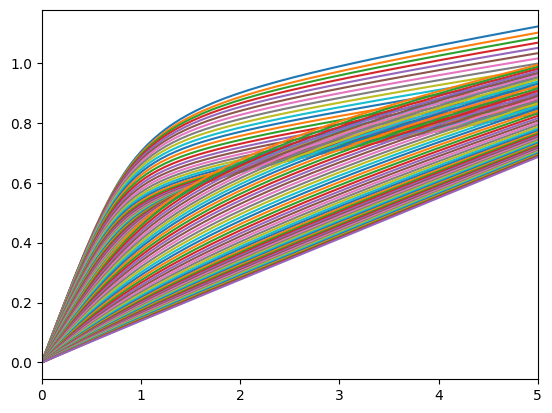
# Plot the consumption functions
print("Consumption functions")
plot_funcs(Agent.cFunc, 0, 5)

Consumption functions

# Number of LifecycleExamples and periods in the simulation.
Agent.AgentCount = 500
Agent.T_sim = 200

# Set up the variables we want to keep track of.
Agent.track_vars = ["aNrm", "cNrm", "pLvl", "t_age", "mNrm"]

# Run the simulations
Agent.initialize_sim()
Agent.simulate()

raw_data = {
    "Age": Agent.history["t_age"].flatten() + birth_age - 1,
    "pIncome": Agent.history["pLvl"].flatten(),
    "nrmM": Agent.history["mNrm"].flatten(),
    "nrmC": Agent.history["cNrm"].flatten(),
}

Data = pd.DataFrame(raw_data)
Data["Cons"] = Data.nrmC * Data.pIncome
Data["M"] = Data.nrmM * Data.pIncome

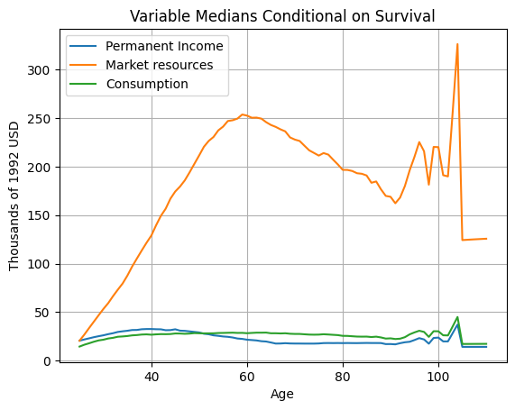
# Find the mean of each variable at every age
AgeMeans = Data.groupby(["Age"]).median().reset_index()

plt.figure()
plt.plot(AgeMeans.Age, AgeMeans.pIncome, label="Permanent Income")
plt.plot(AgeMeans.Age, AgeMeans.M, label="Market resources")
plt.plot(AgeMeans.Age, AgeMeans.Cons, label="Consumption")
plt.legend()
plt.xlabel("Age")
plt.ylabel(f"Thousands of {adjust_infl_to} USD")
plt.title("Variable Medians Conditional on Survival")
plt.grid()