This page was generated from examples/ConsBequestModel/BequestWarmGlowPortfolioType.ipynb.
Interactive online version: . Download notebook.

Warm-Glow Bequest Motive and Portfolio Choice

The BequestWarmGlowPortfolioType extends BequestWarmGlowConsumerType to include portfolio allocation between a risky and riskless asset. Because the model combines two others in HARK, the details of the solution methods are not extensively covered here. Please see our other notebooks on bequest motives and portfolio allocation.

# Initial imports and setup
from time import time
import numpy as np
import matplotlib.pyplot as plt

from HARK.Calibration.Income.IncomeTools import (
    Cagetti_income,
    parse_income_spec,
    parse_time_params,
)
from HARK.Calibration.life_tables.us_ssa.SSATools import parse_ssa_life_table
from HARK.models import BequestWarmGlowPortfolioType, PortfolioConsumerType
from HARK.ConsumptionSaving.ConsBequestModel import init_portfolio_bequest

mystr = lambda number: f"{number:.4f}"

Warm Glow Bequest with Portfolio Allocation Model Statement

Each period, a BequestWarmGlowPortfolioType chooses how much to consume vs save in assets, and how to divide their wealth between a risky and riskless asset. They receive flow utility from consumption according to a CRRA function, and also have a “warm glow” bequest motive that yields additional utility at their passing.

\(\newcommand{\CRRA}{\rho}\) \(\newcommand{\LivPrb}{\mathsf{S}}\) \(\newcommand{\DiscFac}{\beta}\) \(\newcommand{\PermGroFac}{\Gamma}\) \(\newcommand{\Rfree}{\mathsf{R}}\) \(\newcommand{\Risky}{\mathfrak{R}}\) \(\newcommand{\BeqShift}{\xi}\) \(\newcommand{\BeqFac}{\alpha}\)

The model can be written in Bellman form as:

\begin{align*} \text{v}_t(m_t) &= \max_{c_t, s_t} \frac{c_t^{1-\CRRA}}{1-\CRRA} + \LivPrb_t \DiscFac \mathbb{E} \left[ (\PermGroFac_{t+1} \psi_{t+1})^{1-\CRRA}\text{v}_{t+1}(m_{t+1}) \right] + (1-\LivPrb_t) \BeqFac \frac{(a_t + \BeqShift)^{1-\CRRA}}{1-\CRRA} \\ &\text{s.t.} \\ a_t &= m_t - c_t, \\ a_t &\geq 0, \\ s_t &\in [0,1], \\ m_{t+1} &= a_t R_{t+1}/(\PermGroFac_{t+1} \psi_{t+1}) + \theta_{t+1}, \\ R_{t+1} &= s_t \Risky_{t+1} + (1-s_t) \Rfree_{t+1}, \\ (\psi_{t+1},\theta_{t+1}) &\sim F_{t+1}, \\ \Risky_{t+1} &\sim G, \\ \mathbb{E}[\psi] &= 1. \\ \end{align*}

The model is identical to that of the standard RiskyAssetConsumerType but for the addition of the bequest motive term.

Example Parameters for BequestWarmGlowPortfolioType

The default parameters for BequestWarmGlowPortfolioType combine those of BequestWarmGlowConsumerType and PortfolioConsumerType. Thus the “advanced options” for portfolio models are available in this model.

Parameter	Description	Code	Example value	Time-varying?
\(\DiscFac\)	Intertemporal discount factor	DiscFac	\(0.96\)
\(\CRRA\)	Coefficient of relative risk aversion	CRRA	\(2.0\)
\(\Rfree_t\)	Risk free interest factor	Rfree	\([1.03]\)	\(\surd\)
\(\gamma\)	Marginal propensity to consume in terminal period	BeqMPC	\(0.2\)
\(\kappa\)	Consumption function intercept term in terminal period	BeqInt	\(0.1\)
\(\mu_\Risky\)	Mean risky asset return	RiskyAvg	\(1.08\)
\(\sigma_\Risky\)	Standard deviation of log risky asset return	RiskyStd	\(0.18\)
\(N_\Risky\)	Number of equiprobable nodes in risky asset return distribution	RiskyCount	\(5\)
\(\LivPrb_t\)	Survival probability	LivPrb	\([0.98]\)	\(\surd\)
\(\PermGroFac_{t}\)	Permanent income growth factor	PermGroFac	\([1.01]\)	\(\surd\)
\(\sigma_\psi\)	Standard deviation of log permanent income shocks	PermShkStd	\([0.1]\)	\(\surd\)
\(N_\psi\)	Number of discrete permanent income shocks	PermShkCount	\(7\)
\(\sigma_\theta\)	Standard deviation of log transitory income shocks	TranShkStd	\([0.1]\)	\(\surd\)
\(N_\theta\)	Number of discrete transitory income shocks	TranShkCount	\(7\)
\(\mho\)	Probability of being unemployed and getting \(\theta=\underline{\theta}\)	UnempPrb	\(0.05\)
\(\underline{\theta}\)	Transitory shock when unemployed	IncUnemp	\(0.3\)
\(\mho^{Ret}\)	Probability of being “unemployed” when retired	UnempPrbRet	\(0.0005\)
\(\underline{\theta}^{Ret}\)	Transitory shock when “unemployed” and retired	IncUnempRet	\(0.0\)
\((none)\)	Period of the lifecycle model when retirement begins	T_retire	\(0\)
\((none)\)	Minimum value in assets-above-minimum grid	aXtraMin	\(0.001\)
\((none)\)	Maximum value in assets-above-minimum grid	aXtraMax	\(20.0\)
\((none)\)	Number of points in base assets-above-minimum grid	aXtraCount	\(48\)
\((none)\)	Exponential nesting factor for base assets-above-minimum grid	aXtraNestFac	\(3\)
\((none)\)	Additional values to add to assets-above-minimum grid	aXtraExtra	\(None\)
\(K\)	Number of discrete points in risky share grid	ShareCount	\(25\)
\(L\)	Number of times to perform an “augmented” risky share search	ShareAugFac	\(0\)
\((none)\)	Fixed risky asset share, disallowing portfolio choice	RiskyShareFixed	\(1.0\)
\((none)\)	Indicator for whether vFunc should be computed	vFuncBool	\(False\)
\((none)\)	Indicator for whether cFunc should use cubic splines	CubicBool	\(False\)
\((none)\)	Indicator for whether \(F_t\) and \(G\) are independent	IndepDstnBool	\(True\)

Example Implementation of BequestWarmGlowPortfolioType

Just like BequestWarmGlowConsumerType, this model produces more interesting results in a life-cycle setting than for infinite horizon, so let’s specify reasonably plausible parameters in a dictionary.

# Define a life-cycle calibration using HARK tools
birth_age = 22
death_age = 110
adjust_infl_to = 1992
income_calib = Cagetti_income["College"]
income_calib["PermShkStd"] = 0.1
income_calib["TranShkStd"] = 0.1

# Income specification
income_params = parse_income_spec(
    age_min=birth_age,
    age_max=death_age,
    adjust_infl_to=adjust_infl_to,
    **income_calib,
)

# Survival and time specification
liv_prb = parse_ssa_life_table(
    female=False, cross_sec=True, year=2004, age_min=birth_age, age_max=death_age
)
time_params = parse_time_params(age_birth=birth_age, age_death=death_age)

# Put it all together into a dictionary
lifecycle_dict = income_params.copy()
lifecycle_dict["LivPrb"] = liv_prb
lifecycle_dict.update(**time_params)
lifecycle_dict["Rfree"] = lifecycle_dict["T_cycle"] * [1.01]
lifecycle_dict["Risky"] = 1.04
lifecycle_dict["T_sim"] = 80
lifecycle_dict["seed"] = 0
lifecycle_dict["CRRA"] = 5.0

# Combine the life-cycle parameters with the default parameters for the bequest motive model
my_params = init_portfolio_bequest.copy()
my_params.update(lifecycle_dict)
del my_params["constructors"]  # don't overwrite

We’ll use the portfolio allocation model without a bequest motive as a baseline comparison. Note that we’re giving PortfolioConsumerType bequest motive parameters, but they will be ignored.

# Make and solve a baseline consumer type
BaseType = PortfolioConsumerType(**my_params)
t0 = time()
BaseType.solve()
t1 = time()
print("Solving the baseline consumer's problem took " + mystr(t1 - t0) + " seconds.")

Solving the baseline consumer's problem took 3.0891 seconds.

Just like in the bequest model without portfolio allocation, the bequest motive will make the agents want to hold more wealth, so we’ll make two versions with a bequest motive. The first will have the same discount factor \(\DiscFac\) as our baseline agents, and the other will be significantly more impatient (\(\DiscFac = 0.925\)). The latter type’s discount factor is (roughly) calibrated so that their wealth at retirement is similar to the baseline type’s.

# Make and solve a consumer with a bequest motive
BequestType = BequestWarmGlowPortfolioType(**my_params)
t0 = time()
BequestType.solve()
t1 = time()
print("Solving the bequest consumer's problem took " + mystr(t1 - t0) + " seconds.")

Solving the bequest consumer's problem took 3.1393 seconds.

# Make and solve a consumer with a bequest motive who is more impatient
ImpatientType = BequestWarmGlowPortfolioType(**my_params)
ImpatientType.DiscFac = 0.925
t0 = time()
ImpatientType.solve()
t1 = time()
print("Solving the impatient consumer's problem took " + mystr(t1 - t0) + " seconds.")

Solving the impatient consumer's problem took 3.1864 seconds.

Now we can simulate all types’ model and plot the trajectory of wealth over their lifecycle.

# Simulate all types' models, following one cohort without death
t0 = time()
BaseType.initialize_sym(stop_dead=False)
BaseType.symulate()
BequestType.initialize_sym(stop_dead=False)
BequestType.symulate()
ImpatientType.initialize_sym(stop_dead=False)
ImpatientType.symulate()
t1 = time()
print("Simulating all types took " + mystr(t1 - t0) + " seconds.")

Simulating all types took 3.1172 seconds.

# Extract mean wealth profiles for all types
aLvl_base = BaseType.hystory["aNrm"] * BaseType.hystory["pLvl"]
aLvl_bequest = BequestType.hystory["aNrm"] * BequestType.hystory["pLvl"]
aLvl_impatient = ImpatientType.hystory["aNrm"] * ImpatientType.hystory["pLvl"]
A_base = np.mean(aLvl_base, axis=1)
A_bequest = np.mean(aLvl_bequest, axis=1)
A_impatient = np.mean(aLvl_impatient, axis=1)

# Plot the three types' average wealth profiles
age_vec = np.arange(22, 102)
plt.plot(age_vec, A_base, "-b")
plt.plot(age_vec, A_bequest, "-r")
plt.plot(age_vec, A_impatient, "-g")
plt.legend(["Baseline", "Bequest motive", "Beq motive, impatient"], loc=2)
plt.xlabel("Age")
plt.ylabel("Average wealth, 1000's USD")
plt.ylim(0.0, None)
plt.show()

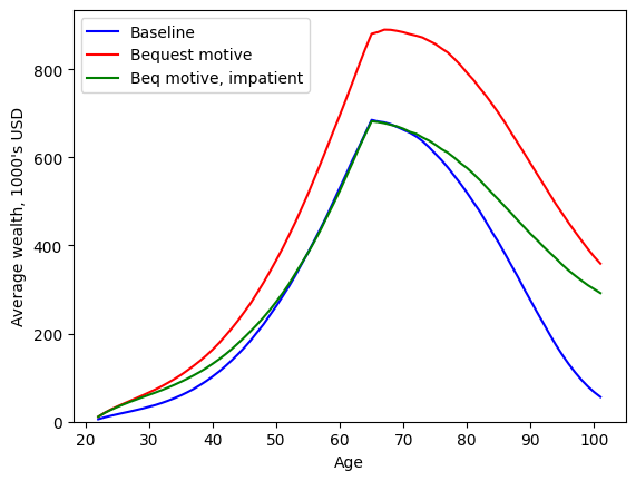
This graph should familiar if you’ve looked at the notebook for BequestWarmGlowConsumerType. The agents want to hold more wealth in old age (i.e. not run down their wealth to zero), so they accumulate more wealth early in life to finance their desire to consume and hold wealth when old. When the discount factor is adjusted so that agents accumulate about the same amount at retirement as in the baseline, we see that they want to decumulate their wealth more slowly, with a positive target wealth ratio even as death becomes increasingly likely.

We can also plot the (aggregate) share of wealth held in the risky asset for each of the three models.

# Extract risky share profiles for all types
risky_assets_base = BaseType.hystory["Share"] * aLvl_base
risky_assets_bequest = BequestType.hystory["Share"] * aLvl_bequest
risky_assets_impatient = ImpatientType.hystory["Share"] * aLvl_impatient
S_base = np.mean(risky_assets_base, axis=1) / A_base
S_bequest = np.mean(risky_assets_bequest, axis=1) / A_bequest
S_impatient = np.mean(risky_assets_impatient, axis=1) / A_impatient

# Plot the three types' share of wealth held in the risky asset
age_vec = np.arange(22, 102)
plt.plot(age_vec, S_base, "-b")
plt.plot(age_vec, S_bequest, "-r")
plt.plot(age_vec, S_impatient, "-g")
plt.legend(["Baseline", "Bequest motive", "Beq motive, impatient"], loc=3)
plt.xlabel("Age")
plt.ylabel("Share of wealth in risky asset")
plt.ylim(0.0, 1.01)
plt.show()

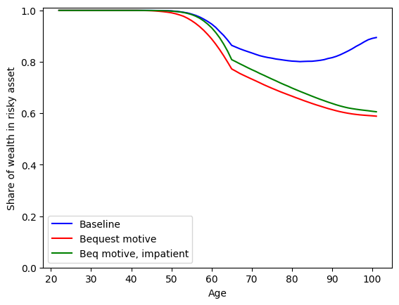
The optimal risky asset share is non-increasing in wealth, so agents with a bequest motive (who run up more wealth) will tend to put a smaller share of that wealth into the risky asset. Early in life, all three types of agent hold (nearly) all of their wealth in the risky asset, as they have many future periods for the higher risky returns to accumulate and “smooth out” the ups and downs of the market. As retirement approaches, the agents anticipate that a large share of their consumption will be financed through their wealth holdings, and they begin to scale back their risky investments to reduce future consumption fluctuations. This pattern continues through retirement except for the baseline agents, who run their wealth down so far that the downward slope of the risky share function (w.r.t. wealth) overcomes the prudence effect of consuming from wealth, and they increase their risky allocation late in life.